The success of just-in-time compilers is based on their ability to
specialize code at run time. It allows them to dynamically observe
the execution of a program and optimize code for properties of the
current program state. Just-in-time compilation is the blackest
of arts in language implementation; the initiation rituals
include brutal debugging sessions and an oath to pierce all
abstractions. While I enjoy flipping bits, I still believe that at least
some of the suffering is avoidable and building just-in-time
compilers could be a topic as precisely documented as any.
Hence, a main motivation for writing this dissertation is to
digest some of this black magic and capture it in simple
and precise terms. This includes the following contributions:
A calculus featuring a precise description of speculative
optimizations with dynamic deoptimization.
Context dispatch, a generic approach for specializing
code up to a context of dynamically checked assumptions.
A case study of a realistic language implementation
following these implementation recipes, featuring an
intermediate representation to analyze and compile R
programs.
This dissertation consists of two parts. First, the models and
theoretical findings are presented. The goal of that part is to
explain how and why dynamic optimizations work, how dynamic
information can be used for optimizations, and how assumptions
interact in with static compiler optimizations. Additionally, it is
discussed how the models combine and how complete they are
with regards to a full-blown language implementation. Secondly,
Ř is described and evaluated. Ř is an implementation of the R
language, following the recipes introduced by the first part. This
allows us to connect and evaluate the designs with a realistic
implementation.
Acknowledgments
Along the way many, many people helped me shape raw
curiosity into a useful tool and empowered me to write this
dissertation.
Most importantly, my heartfelt thanks for the unconditional
support go to my adviser, Jan Vitek. I will truly miss the joy of
working with you.
Many thanks to my plentiful and awesome co-authors and
co-conspirators, including Aurèle Barrière, Guido Chari, Aviral
Goel, Jakob Hain, Jan Ječmen, Filip Křikava, Sebastián Krynski,
Paley Li, Petr Maj, Gabriel Scherer, Andreas Wälchli, Ming-Ho
Yee.
Without the encouragement and patience of many mentors I
would not have started this endeavor. Most prominently, thank
you Toon Verwaest and Oscar Nierstrasz for sending me down
this rabbit-hole. Thanks for teaching me everything about
compilers and VMs to Daniel Clifford, Tomas Kalibera, Ben
Titzer.
I also thank the PLISS attendees, who shall remain anonymous,
for openly sharing that every PhD comes with its fair share of
doubt and resignation.
Last but not least I am very grateful to my committee for
engaging with my work and helping me better understand and
explain it. Thank you Amal Ahmed, Mathias Felleisen, Filip
Pizlo, and Steve Blackburn. In particular Matthias for your
dedication.
Thank you to all the people I love for everything we have and
still will experience. See you in the streets.
Just-in-time compilers are omnipresent in today’s technology
stacks. The performance of the code they generate is central to
the growing adoption of languages with dynamic features
such as code loading, extensible objects, monkey-patching,
introspection, or eval. These kind of features render precise
static analysis impossible and lead to a wide range of possible
behaviors, even in seemingly benign programs. To resolve this
issue compilers specialize programs at run-time according to
observed behaviors — they identify likely invariants and
optimize1
assuming the invariants hold. For instance,
in prototype based languages classes of likely similar
objects are identified using hidden classes [Chambers and
Ungar, 1989],
duck-typing and late bound call targets are made static
by speculating on the stability of the dynamic call-graph
and monomorphized by splitting [Hölzle, Chambers,
and Ungar, 1991],
Most optimizations in just-in-time compilers are based in some way on
the premise that, from the vast range of possible behaviors only
some will be exercised by any particular execution of a program.
Specializing code to those particular behaviors has been
fundamental in making dynamic languages practical in large
applications. These kind of optimizations involve forming
assumptions about likely behaviors, that are expected to hold
true at run-time. Typically the assumptions are based on
profiling data, gathered either from the current process or from
previous invocations. This is a common practice, even utilized in
ahead-of-time compilers, where it is known as profile guided
optimizations. The advantage in a just-in-time scenario is that
specialization can be explored lazily, generating only code that is
actually needed, in contrast to the ahead-of-time case, where the
generated code must handle all possible behaviors all the time. A
fundamental problem in just-in-time compilation is therefore how
to leverage dynamic analysis, i.e., an incomplete recording of the
past behavior, for optimizations? In particular, how to speculate
and specialize code for likely invariants, while still safely
and efficiently handling the case where they turn out not to
hold. The implementation thereof is often scattered around
different components of the language implementation; for
instance, devirtualization in a language with class loading
relies on the interplay of collecting a dynamic call-graph
in the runtime, optimizing under the assumption that it is
stable and retiring code invalidated by the class loader, while
handling the cases where the invalidated code is still being
executed.
1.1 Motivation
In this area of run-time optimizations, there is a lack of
well-documented and re-usable techniques. Specialization
is typically ad-hoc, tied to peculiarities of the language or
implementation, and often even distinct for different properties in
the same system. For instance the specialization approach taken
by Julia [Bezanson, Karpinski, Shah, and Edelman, 2012]
requires a language with multi-method dispatch, the one by
Truffle [Würthinger, Wimmer, Wöß, Stadler, Duboscq,
Humer, Richards, Simon, and Wolczko, 2013] relies on their
language implementation style using self-specializing AST
interpreters. Speculative optimizations in particular are poorly
documented and mistaken for an implementation detail on how
to rewrite stack frames. This gap in the literature leads to
island-solutions for each language and a reluctance by some
language implementers to include speculation in their compiler.
The reluctance is the result of a poor understanding of the
underlying program transformations and missing off-the shelf
techniques.
Speculation in particular is iconic for just-in-time compilation.
Having a compiler available at run-time allows for multiple
attempts at producing optimal code. This allows for aggressive
optimization strategies, where code is expected to be wrongly
optimized sometimes, but then subsequently and transparently
replaced by updated and fixed code. Speculative optimizations
stand out from other techniques by their ability to — at arbitrary
program locations — exclude some parts of the source code from
the code being optimized. This is achieved by guarding against
unexpected behaviors with run-time checks and bailing out of the
optimized code, back to the source code, if these guards
fail. It follows that speculative optimizations allow us to
trim down the vast range of possible behaviors and instead
optimize and even analyze just for the expected ones. It also
means, that some form of recovery action is necessary in the
unexpected case. We refer to that action as deoptimization
and it relies on some form of execution state rewriting by
the underlying runtime, such as on-stack-replacement or
stack-switching.
A non-speculating specialization on the other hand involves
upfront splitting of the control-flow on a property. I will
refer to them as contextual optimizations, as they specialize
code to certain predicates over the program state. Often
contextual optimizations result in the duplication of the code
being optimized. Real-world examples include multi-method
dispatching on argument types in Julia, where each function
signature discovered through dispatch leads to a new function
being compiled and optimized. Or, optimizations involving
tail-duplication, such as message splitting in SELF, where the
control-flow within a function is split on the type of a result of a
message send to produce optimized continuations for expected
dynamic types.
As a concrete example, consider a code fragment S, which is
part of a lager program, and shall be specialized to a certain
runtime context. For instance the fragment S could have a
free variable x and the goal is to provide a particularly fast
implementation for, say, the cases where x is 42. A fragment could
be a function body, but also a smaller or bigger piece of code. Let’s
assume S is the following expression:
if(!is.numeric(x)||x==0) error() else 1/x
For a simple non-speculating optimization we start with a
transformation to duplicate the fragment into if (x == 42)then S else S. This allows us to optimize each clone of S
independently under the contextual information whether x == 42
holds. Within the then branch, the compiler can assume x == 42
to be part of the static optimization context, and conversely within
the else branch x != 42.
Now let us contrast this approach with a speculative
optimization. In that case we simply state assert(x == 42); S.
For expressions dominated by the assertion, the fact x == 42 is
again part of the static optimization context. The case where that
assumption does not hold, is not part of the code emitted by such
a compiler.
In summary, a speculative optimization means that the
compiler can simply assume a likely invariant at a certain program
location, and the unexpected case falls outside the compilation
unit. Under speculative optimizations we also allow instructions
being executed optimistically and work being done that has
to be discarded or even reverted if the assumption fails. A
non-speculative optimization on the other hand produces code that
cannot be invalidated. It is still possible to optimize for dynamic
properties, though the properties are used in a non-speculative
way.
Example
Consider the following vector access function in R
at<-function(x,y) x[[as.numeric(y)]]
which converts the y argument to a number and then uses that
number as an index into argument x. Assume we call the
function with three different kinds of arguments as follows:
In the first two cases the type of the argument is known at the
call site. This does not hold for the third case, because R
evaluates arguments by need; pos() is only invoked, when the y
argument is accessed for the first time, which happens during the
execution of at. If we were to clone the function at and optimize
it for different types of arguments, we can specialize it for
three distinct cases: number[n] × number for the call-site at
line 3, number[n] × string at line 5, and number[n] ×any at line 8. The first two signatures directly lead to well
optimized versions — at the source level they would look like:
at_2<-function(x,y){ y<-as.numeric(y) if(is.na(y)) NA else at_1(x,y) }
The third case does not lend itself to any useful optimizations,
since at the call-site it is unclear what the expression pos()
eventually returns (excluding inter-procedural analysis for now).
This is where speculation comes into play, and type-feedback from
previous runs can be employed to narrow down the behavior to
what we expect from the past. To make lazy evaluation specific,
we’ll mark the position where arguments are evaluated with force.
After forcing the argument expression, we can then speculate on
its type and shape:
In case our assumptions are wrong, the assume instruction is
supposed to fall back to the source version of this function. It
allows us to ignore unlikely cases, i.e., in this case most of the
implementation of vector access, which would have to deal with
different vector types, indexing modes and possible errors. Of
course for that to actually work, assume is more complicated than
an assertion and more meta-data is required than is shown
here.
Questions
An efficient implementation of a dynamic language must use
information only available at run-time to optimize code. In
particular this information is incomplete and changes over time.
There are fundamentally two approaches to this problem, one is to
speculate on likely properties and fall-back otherwise, the other is
to somehow split control-flow on properties, which are checked
up-front. Both of these approaches present problems and open
questions.
Speculation
The goal of speculation is, that a compiler can base optimizations
not only on static facts, but also on likely invariants. Should a
speculation turn out to be incorrect for a particular execution,
then the optimized code is discarded and the execution switches
back to unoptimized code on-the-fly. But, what does it entail to
bail out of wrongly optimized code that is currently being
executed, i.e., to deoptimize code with active stack frames?
Program counters must be updated, optimized execution state
rewritten into corresponding unoptimized state, potentially
switching from native to interpreted code, and some parts of the
unoptimized state might not even exist and have to be synthesized
and materialized. The mechanism is typically relegated to
implementation details that are neither clearly abstracted nor
documented, and scattered around different levels of the
implementation. Is there a formal and transferable way to model
speculation? How can compiler correctness be stated in the
presence of speculation? When are two versions compiled
under different assumptions equivalent? How do traditional
optimizations have to be adapted? Does deoptimization inhibit
optimizations?
Specialization
There are situations where it is beneficial to optimize code by
specializing it to multiple scenarios. For instance if profile data
suggests that a particular variable alternatively holds one of
two unrelated dynamic types, then it makes sense to split
control on that type and optimize for the two continuations
separately. In other words, the aim of specialization is to split
code, such that contextual information about the current
program state can be used for optimizations. Many existing
splitting and customization techniques fall under this category
and implementations use different approaches to generate
code specialized to certain properties of the program state.
Given such a fragmented space, is there a unified or unifying
technique to describe and implement specialization? How can
a language implementation be structured to benefit from
specialization? Can specialized code be shared between compatible
uses and contexts? What does it mean for contexts to be
compatible? How does specialization interact with speculation?
How can the generation of specialized code be deferred as much
as possible, such that more dynamic information can be
considered.
1.2 Thesis
This dissertation presents a framework for soundly injecting
assumptions into the optimizer of a just-in-time compiler. First,
speculative optimizations with deoptimization as fallback
mechanism are formalized in the sourir model. Sourir’s assume
instruction enables optimizations based on arbitrary assumptions
at any point. Second, context dispatch provides a generic approach
for splitting on properties checked at run-time. Context dispatch
allows to optimize functions lazily, up to the actually encountered
contexts of assumptions, which act like static optimization
contexts in an ahead-of-time compiler. I will defend the thesis
that
Assume and context dispatch provide the basis for
optimizations based on run-time assumptions in a
competitive just-in-time compiler.
To understand that statement I will briefly introduce the
two models, summarize their contributions, and explicit the
claims.
, is a
simple abstraction for speculative optimizations that allows for
formal reasoning on speculation at the IR level. It makes the
following contributions:
a semantic for deoptimization points, assumptions,
deoptimization metadata, and the key invariants
required for speculative optimizations;
correctness proofs for speculative optimizations and
classical optimizations in the presence of speculation; and
the assume instruction for speculation that can be easily
integrated in a compiler IR.
,
unifies how a runtime system can exploit contextual information
and provides a simple approach to structure a just-in-time
compiler around code specialization. It allows a compiler to
specialize fragments of code up to a context of assumptions, and
the specialized fragments to be shared between compatible
contexts. The contributions are how to
add dynamic information to the static optimization
context of a compiler and combine static and dynamic
analysis for specialization;
avoid over-specializing and support sharing of code; and
efficiently dispatch to an optimal version under the
current program state.
Sourir and context dispatch complement each other. I will also
introduce a combined deoptless deoptimization strategy using
context dispatch.
Claims
This thesis presents Ř, a bug-compatible implementation of
the R language with a JIT compiler. R’s dynamic nature and
lazy evaluation strategy requires the optimizer to be able to
optimistically speculate and specialize. The implementation effort
is presented in
, which also covers those particularities of
the R language that make it particularly resilient to optimizations.
Ř uses a context dispatch system, and the optimizing compiler in
Ř has an IR that is based closely on sourir. Ř shows that these
two pieces of theory provide blueprints for building a language
implementation with competitive performance. In particular in Ř
the following claims are validated:
The two approaches provide specializations on dynamic
information in all important situations. The optimizing
compiler in Ř uses dynamic information only in the
form of assume instructions or optimization contexts
from context dispatch. This claim is substantiated in
chapter 4, which describes how sourir and context
dispatch translate into the concrete implementation
and how this implementation relies only on these two
mechanisms for incorporating dynamic information.
The optimizer is competitive. It significantly outperforms
the Ř bytecode interpreter, the GNU R bytecode
interpreter, and is comparable to Oracle’s JIT
compiling FastR, but with faster warmup behavior.
The performance evaluation in chapter 5 shows which
assumptions and contexts are required for Ř to speed
up R programs.
Non-Claims
I want to stress upfront that sourir and context dispatch do not
cover the entirety of the implementation. This dissertation focuses
on the optimizing compiler. In particular the main focus is on the
middle-end of a JIT and optimizations on its IR as enabled by
dynamic information. Other details are important for a good
implementation, such as efficient profile collection, a fast garbage
collector, a native backend, or a good interpreter. Sourir and
context dispatch co-evolved with Ř and were instrumental in my
own understanding of key aspects of JIT compilation. The actual
implementation goes beyond these building blocks — on the one
hand it features extensions for practical reasons, and on the
other hand many more parts are necessary for a complete
language implementation. These extensions are discussed less
formally, when presenting the implementation. A complete model
and potentially a verified JIT implementation remain future
work.
Structure
This thesis is structured as follows. The two main contributions
are presented in chapter 2 and chapter 3. The former presents a
formalization of speculative optimizations and discusses the
relationship of the model with implementations. The latter focuses
on specialization using context dispatch and related applications.
To validate my claims chapter 4 presents how these contributions
are usable in a real-world implementation called Ř and chapter 5
shows that Ř is competitive. chapter 6 concludes and presents
future work.
Publications
The Ř virtual machine is available and developed as free software
at ř-vm.net.
The text of this dissertation is based or borrows from the following
peer-reviewed publications:
Many just-in-time compilers support some form of speculative
optimization to avoid generating code for unlikely control-flow paths.
For instance the prevalent polymorphism in a dynamic language
causes even the simplest code to have non-trivial control flow.
Consider the JavaScript snippet (example by Bebenita, Brandner,
Fahndrich, Logozzo, Schulte, Tillmann, and Venter [2010]):
for(vari=0;i<a.length-1;i++){ vart=a[i]; a[i]=a[i+1]; a[i+1]=t; }Listing 2.1:Shift
in
JavaScript
Without optimization one iteration of the loop executes 210
instructions; all arithmetic operations are dispatched and
their results boxed. If the compiler is allowed to make the
assumption it is operating on integers, the body of the loop
shrinks down to 13 instructions. As another example, most
Java implementations assume that non-final methods are not
overridden. Speculating on this fact allows compilers to avoid
emitting dispatch code [Ishizaki, Kawahito, Yasue, Komatsu, and
Nakatani, 2000]. Newly loaded classes are monitored, and any
time a method is overridden, the virtual machine invalidates code
that contains devirtualized calls to that method. The validity of
speculations is expressed as a predicate on the program state. If
some program action, like loading a new class, falsifies that
predicate, the generated code must be discarded. To undo an
assumption, an implementation must ensure that functions
compiled under that assumption are retired. This entails replacing
affected code with a version that does not depend on the invalid
predicate and, if a function currently being executed is found to
contain invalid code, that function needs to be replaced on
the fly. In such a case, it is necessary to transfer control to
a different version of the function, and in the process, it
may be necessary to materialize portions of the state that
were optimized away and perform other recovery actions.
In particular, if the invalidated function was inlined into
another function, it is necessary to synthesize a new stack
frame for the caller. This is referred to as deoptimization, or
on-stack-replacement, and is found in most industrial-strength
compilers.
Speculative optimization gives rise to a large and
multi-dimensional design space that lies mostly unexplored. First,
compiler writers must decide how to obtain information about
program state. This can be done ahead-of-time by profiling,
just-in-time by sampling or instrumenting code. Second,
they must select which facts to record. This can range from
information about the program, its class hierarchy, which packages
were loaded, to information about the value of a particular
mutable location in the heap. Finally, they must decide how to
efficiently monitor the validity of speculations. While some
points in this space have been explored empirically, existing
systems have done it in an ad hoc manner that is often both
language- and implementation-specific, and thus difficult to
transfer.
The model shown here has a focused goal. The aim is to
demystify the interaction between compiler transformations and
deoptimization. When are two versions compiled under different
assumptions equivalent? How should traditional optimizations be
adapted when operating on code containing deoptimization points?
In what ways does deoptimization inhibit optimizations? The
assume model gives compiler writers the formal tools they need
to reason about speculative optimizations. To do this in
a way that is independent of the specific language being
targeted and of implementation details relative to a particular
compiler infrastructure, we have designed a high-level compiler
intermediate representation (IR), named sourir, that is adequate
for many dynamic languages without being tied to any one in
particular.
A sourir program is made up of functions, and each function
can have multiple versions. We equip the IR with a single
instruction, named assume, specific to speculative optimization.
This instruction has the role of describing what assumptions are
being used to perform speculative optimization and what
information must be preserved for deoptimization. It tests if those
assumptions hold, and in case they do not, transfers control to
another, less optimized version of the code. Reifying assumptions
in the IR makes the interaction with compiler transformations
explicit and simplifies reasoning. The assume instruction is more
than a branch: when deoptimizing it replaces the current stack
frame with a stack frame that has the variables and values
expected by the target version, and, in case the function was
inlined, it synthesizes missing stack frames. Furthermore,
unlike a branch, its deoptimization target is not considered by
the compiler during analysis and optimization. The code
executed in case of deoptimization is invisible to the optimizer.
This simplifies optimizations and reduces compile time as
the analysis remains local to the version being optimized and
the deoptimization metadata is considered to be a stand-in for the
target version.
As an example consider the loop from Listing 2.1. A possible
translation to sourir is shown in Figure 2.1 (less relevant code
elided). Vbase contains the original version. Helper functions Get
and store implement JavaScript (JS) array semantics, and
the function add implement JS addition. Version Vnative
contains only primitive sourir instructions. This version is
optimized under the assumption that the variable a is an
array of primitive numbers, which is represented by the first
assume
instruction. Further, JS arrays can be sparse and
contain holes, in which case access might need to be delegated
to a getter function. For this example HL denotes such a
hole. The second assume instruction reifies the compiler’s
speculation that the array has no holes, by asserting the
predicate t≠HL . It also contains the associated deoptimization
metadata. In case the predicate does not hold, we deoptimize to a
related position in the base version by recreating the variables
in the target scope. As can be seen in the second assume,
local variables are mapped as given by the so called varmap
[i= i ,j = i+ 1 ]; the current value of iis carried over
into the target frame’s i, whereas variable j has to be
recomputed.
To visualize the approach let us consider an abstract graph of
the execution. The speculative optimization appears as shown
in Figure 2.2, gray boxes representing function versions.
Figure 2.2:Speculation
Calling the function invokes the speculatively optimized
version. If a dynamic guard fails, then a deoptimization happens,
we transfer execution to the target version, into the middle of the
function at deopt, discarding the optimized code.
2.1 On-Stack Replacement
Before going into details about how to correctly create and use the
assume
instruction in the compiler IR, this section takes
a step back and presents the underlying implementation
techniques and identifies the different pieces in a real-world
deoptimization. This includes a preview of how to eventually lower
an assume instruction to something a CPU can execute. In general
the relevant implementation technique is known as on-stack
replacement. OSR refers to an exceptional transfer of control
between two versions of a function. It is employed by just-in-time
compilers in situations where a function can or has to be replaced
at once, without waiting for it to exit normally. To the user, this
exchange is not observable, the new function transparently picks
up where the old one stopped. On-stack refers to the fact that the
involved functions have active stack frames that need to
be rewritten. OSR is an umbrella term used in literature
and practice to describe exceptional transfer of control for
different reasons and using different kind of mappings between
stack frames or program states. The term deoptimization and
on-stack replacement are often used interchangeably. Although
their meanings overlap, we should be more precise in their
use.1
The term deoptimization highlights the fact, that optimizations
are being undone. A deoptimization transfers control from a
speculatively optimized version with a failing assumption, to a less
speculatively optimized version, undoing the failing assumption.
On the other hand, the term OSR focuses on the implementation
technique, whereby stack-frames are rewritten. OSR can be used
for other applications, such as implementing exceptions, or
tiering-up, i.e., changing from a less to a more optimized
version. Similarly, deoptimization can be implemented without
OSR, for instance by relying on a execution environment
with support for stack-switching, or simply using tail-calls
and lazy replacement. The latter strategy is employed by
Ř.
As shown in the previous section, speculative optimizations
and in particular deoptimization, needs a way of exiting
and entering functions in the middle of execution, with low
performance impact on the case where the guards hold. When the
guard fails, then instead of continuing normally, the function is
exceptionally terminated and replaced with the unoptimized
baseline function, as visualized in Figure 2.2. A correct
deoptimization requires the system to extract the state of
the optimized function, transform it into a corresponding
unoptimized state and then materialize it to continue the
execution.
Definitions
We call functions that should be exited origins and their
replacements targets. Each function has an execution state, or stackframe, that is dependent on the code format but typically consists
of at least the position in the code and the values of local
variables. The format of origin and target can be vastly different if,
for instance, one of them is interpreted and the other runs natively.
A mapping between states captures the steps needed to rewrite
origin states to target states. Since both origin and target are
derived from the same source code, we sometimes use the term
source to refer to the common ancestry of various compiled code
fragments.
shows an idealized OSR that (a) extracts
the state of the origin, (b) maps it to the source, (c) maps it
to the target, and finally (d) materializes the target state.
Figure 2.3:Parts of an OSR event
Origin and target do not need to be constrained to a single
stack frame and a single function. For example when exiting an
inlined function, one origin function maps to multiple target
functions. In other words, the stack frame of the origin needs to be
split into multiple target stack frames.
OSR has been described as black magic due to the
non-conventional control-flow that it introduces. A significant part
of the complexity comes from the fact that most implementations
do not provide clean abstractions for OSR. For example,
extracting and rewriting the program state, i.e., steps (a) and (b)
in Figure 2.3, are often not separated cleanly. Both of these two
steps provide challenges, but for different reasons. Extracting the
program state is challenging due to low-level concerns. We need
very fine grained access to the internal state of the computation at
the OSR points. This access has to be provided by the backend of
our compiler, e.g., by exposing how the execution state is mapped
to the hardware or the interpreter. On the other hand, mapping
the extracted program state to a target state, i.e., creating a
correct varmap, relies on the optimizer providing the required
information.
Simplifications
In practice, many implementations follow a simplified design
combining (b) and (c) into one mapping that translates directly
from one state to another. This works particularly well, if the
compiler of one end of the OSR uses the code of the other end of
the OSR as source code. For instance a typical implementation
uses the bytecode of the first tier interpreter as the source code of
the optimizing native compiler:
In this architecture, there is only one compiler and one
compilation direction between the two ends of the OSR. In other
words, the origin code is the source code of this compiler, therefore
the mapping takes just one step, from native to bytecode (BC). On
the other hand, in the case where both ends of the OSR are
compiled from some common source code, the mapping of
execution states has two steps, as it needs to pass through
the original source. Given the following two compilation
tiers:
the second compilation mandates a mapping that lifts
the state from an origin (native) state to a source state,
the first compilation a mapping that lowers it to a target
(BC) state. Therefore, the generic model is important in
cases where OSR transitions from optimized to optimized
code.
In sourir, the origin and target state of a deoptimization
have the same representation. In other words the varmap
corresponds to (c), the mapping (b) is the identity, since
source and origin are identical. Furthermore (a) and (d) are
trivial, since our execution states are semantic states of the
sourir IR. This simplification was made to focus on the main
problem of creating and maintaining a correct mapping for
deoptimization.
Directions
If OSR jumps from optimized to unoptimized code, we call it
OSR-out, or deoptimization, when it is used to bail out of
failing speculative optimizations. As a simple example, if the
user debugs optimized code with constant-folding applied to,
then deoptimization can be used to restore the constant
values. If OSR jumps from unoptimized to optimized code,
we call it OSR-in or tiering up. This is useful, for instance,
when the program is stuck in a long-running loop. In the
general case where it jumps from optimized to optimized
code, both apply and we simply call it OSR. Typically OSR
cannot happen at arbitrary locations; we call the possible
locations OSR exit or OSR entry points. OSR is general as it
allows to undo arbitrary transformations. When OSR is used
to transition between different optimization levels, it must
be transparent, i.e., deoptimization becomes part of the
correctness argument for optimizations. In turn, deoptimization
enables compiler transformations that would otherwise be
unsound.
Implementation Choices for OSR-out
The lowest overhead to peak performance for OSR exit
points can be achieved by extracting the execution state
by an external mechanism. Typically, at a defined location
execution is conditionally stopped and control transferred to an
OSR-out implementation, e.g., by tail-calling it. The OSR-out
implementation needs metadata produced by the compiler that
describes how the execution state can be retrieved from the
registers and native run-time stack. This is only possible with
fine-grained control over the code layout produced by the
native backend. For efficiency, certain implementations will
go to great lengths to implement the conditional guard of
assume
instructions such that it has the lowest overhead on the
fast-case. This can go as far as compiling it to a nop, that
will be patched inline, in case some external condition is
invalidated. A simpler alternative implementation is to pass all the
required state as arguments to a dedicated OSR-out primitive
function. This approach generates more code, as the state
extraction is effectively embedded into the emitted code but
is easy to implement and efficient in case deoptimization
triggers.
Simplified OSR-in
Whereas OSR-out relies on the ability to extract the
source execution state at many locations, OSR-in is simpler.
While one could arrange for OSR-in to enter optimized code
in the middle of a function, these entry points would limit
optimizations and would not be easy to implement, in particular if
using an off-the-shelf code generator such as LLVM. Instead,
one can compile a continuation starting from the current
program location to the end of the current function. This
continuation is executed once and on the next invocation
the function is compiled a second time from the beginning
of the function. This approach simplifies the mapping of
execution states, as there is only one concrete state that needs
to be mapped instead of multiple abstract states at every
potential entry point. The current state is simply passed as an
argument to the continuation. This is a popular implementation
choice.
2.2 Contributions and Limitations
We now turn our attention back to the optimizations. From now
on this chapter stays at the abstraction level of a compiler
intermediate representation. In that representation we develop
notions and techniques to correctly produce and maintain the
mapping (c) from Figure 2.3. We prove the correctness of a
selection of traditional compiler optimizations in the presence of
speculation; these are constant propagation, unreachable code
elimination, and function inlining. The main challenge for
correctness is that the transformations operate on one version in
isolation and therefore only see a subset of all possible control
flows. We show how to split the work to prove correctness between
the pass that establishes a version-to-version correspondence and
the actual optimizations. Furthermore, we introduce and prove the
correctness of three optimizations specific to speculation, namely
unrestricted deoptimization, predicate hoisting, and assume
composition.
Our work makes several simplifying assumptions. We ignore
the issue of generation of versions: we study optimizations
operating on a program at a certain point in time, on a set
of versions created before that time. We do not model the
low-level details of code generation. Sourir is not designed for
implementation, but about reasoning support for existing or new
JIT implementations.
Most importantly, in sourir the origin and target state of a
deoptimization have the same representation. This simplification
was made to focus on the main problem of mapping the
states. For an actual implementation the target state most
likely has a different representation. For instance in Ř, and
similarly in Java, the target is the bytecode interpreter. In
other words deoptimization materializes program states of
an interpreter — the deoptimization target is a bytecode
offset, the target values are placed on the operand stack
of the interpreter, and so on. We refer to chapter 4 for an
example of how to bridge this gap. If we compare the varmaps
of this implementation with the sourir model, then what
changes are the left-hand sides of the mapping. Instead of
creating a sourir environment of local variables, the target
state for instance consists of an operand stack. For instance,
instead of [i= i ,j = i+ 1 ], the varmap might be
[stack= ⟨i ,i+ 1⟩]. Since the optimizer operates only on the
right-hand sides of the varmaps, the changes affect only the
front-end of the full compiler and do not affect the results from
this chapter.
Finally, the assume IR might be lowered to some more
optimized execution format, say a native binary. Lowering assume
instructions is outside the scope of this chapter. The issues in
doing so are similar to lowering a call instruction, but often great
additional care is taken for the instruction to have as little
overhead as possible if the guarding condition holds, as we expect
this to be the default case. How the proofs can be extended to
include native code is future work.
2.3 Related Work
OSR for deoptimization was pioneered in SELF by Hölzle,
Chambers, and Ungar [1992]. At first, the idea was simply to
deoptimize code to provide a source-level debugging experience. In
that sense, it was a speculative optimization on the assumption
that debugging is not used. Soon the idea was applied to
speculatively optimize for all kinds of assumptions, from the
stability of class hierarchies [Paleczny et al., 2001] to unlikely
behavior in general [Burke, Choi, Fink, Grove, Hind, Sarkar,
Serrano, Sreedhar, Srinivasan, and Whaley, 1999], and providing
more and more flexibility to the optimizer in the presence of
deoptimization [Soman and Krintz, 2006]. We are reaching the
point where deoptimization is an off-the-shelf technique that
more and more compilers are relying on for diverse purposes
[Odaira and Hiraki, 2005, Schneider and Bolz, 2012, Duboscq,
Würthinger, and Mössenböck, 2014, Stadler, Welc, Humer,
and Jordan, 2016, Ap and Rohou, 2017, Qunaibit, Brunthaler,
Na, Volckaert, and Franz, 2018, Pizlo, 2014]. The common idea is
that deoptimization leads the control-flow back to less optimized
code. Most modern just-in-time compilers rely on speculative
compilation to generate code for a subset of the possible
behaviors of a function. The drawback of speculation is that
it does not scale well with very dynamic behavior, as the
speculation applies indiscriminately. Another drawback of
speculation is that deoptimization is costly, as the compiler
needs to add and maintain safe-points which inhibit some
optimizations.
OSR-in (i.e., using OSR to transition from a less to a
more optimized version) was first described by Hölzle and
Ungar [1994a] in their recompilation strategy. When a small
function is invoked often, they rather recompile the caller
and replace it using OSR-in. SELF, being an interactive
system, was concerned with compilation pauses. Especially with
splitting-based optimizations that could lead to an explosion of
code size. Chambers and Ungar [1991] address this issue by
identifying uncommon source-level control-flows and deferring
their compilation. Suganuma, Yasue, and Nakatani [2003] describe
the natural extension of this idea where the deferred compilation is
implemented by means of OSR. The Jikes RVM extensively relied
on OSR-in for profile-driven deferred compilation as described by
Fink and Qian [2003]. Deferred compilation can be understood as
a speculative optimization that assumes an unlikely source-level
branch is not taken.
Most compilers use an architecture, where OSR transitions are
only possible between versions linked by one compilation step. A
notable exception are Wimmer, Jovanovic, Eckstein, and
Würthinger [2017] who present OSR from optimized to optimized
code. The goal is to use an optimizing compiler as the baseline
compiler. They note that it requires “a two-way matching of two
scope descriptors describing the same abstract frame.” In terms of
our definitions in the previous section, this corresponds to
an origin and a target state, which are related through a
corresponding source state.
On the other hand, the one-step architecture is sometimes
further simplified by the optimizer having the same source
and target language. For example Béra, Miranda, Denker,
and Ducasse [2016] advocate a VM architecture that uses a
bytecode-to-bytecode optimizer, or Essertel, Tahboub, and
Rompf [2021] implement OSR as source-to-source transformation.
Wang, Blackburn, Hosking, and Norrish [2018] argue for a
common low-level code format for all optimization levels and a
low-level virtual machine, the Mu micro VM [Wang, Lin,
Blackburn, Norrish, and Hosking, 2015], to efficiently execute this
code. OSR as a mechanism is provided by the virtual machine,
e.g.,, by means of a swapstack primitive operation. A similar
argument is made by Desharnais and Brunthaler [2021].
As a result OSR is trivial to implement on top of such an
architecture, since all the implementation complexity has
to be handled already by the lower layer. Note however,
that such a one-language approach, while simplifying the
implementation, does not simplify the creation of a correct
mapping for undoing optimizations. The problem of keeping two
versions’ execution states synchronized across optimization
passes still applies. That’s why the assume model in this
dissertation also makes this one-language simplifying assumption,
because it aims to solve the problem of correct mappings in
isolation.
Previous work has made in-roads in demystifying JIT compilation.
Myreen [2010] presents a verified JIT compiler from a stack-based
bytecode to x86. The work focuses on self-modifying code, which
modern JITs typically do not use anymore. The reasons are that
for security reasons memory cannot be writable and executable at
the same time, plus invalidating instruction caches is an
expensive operation. What is not covered by Myreen are compiler
optimizations and any kind of speculation, deoptimization, or
specialization.
Guo and Palsberg [2011] discussed the soundness of
trace-based compilers. When optimizing a trace, the rest of the
program is not known to the optimizer, so optimizations
such as dead-store elimination are unsound: a store might
seem useless in the trace itself, but actually impacts the
semantics of the rest of the program. On the other hand, free
variables of the trace can be considered constant for the entire
trace.
D’Elia and Demetrescu [2018] present an LLVM extension
with OSR exit and entry points, and their interaction with
optimization passes. Béra et al. [2016] present a verifier for a
bytecode-to-bytecode optimizer. By symbolically executing optimized
and unoptimized code, they verify that the deoptimization
metadata produced by their optimizer correctly maps the
symbolic values of the former to the latter at all deoptimization
points.
There is a rich literature on formalizing compiler optimizations.
The CompCert project [Leroy and Blazy, 2008] for example
implements many optimizations, and contains detailed proof
arguments for a data-flow optimization used for constant folding
that is similar to ours. In fact, sourir is close to CompCert’s
RTL language but comes with versions and assumptions.
There are formalizations for tracing compilers [Guo and
Palsberg, 2011, Dissegna, Logozzo, and Ranzato, 2014], but we
are unaware of any other formalization effort for speculative
optimizations in general.
2.4 Speculation in a Nutshell
This section introduces our IR and its design principles. We first
present the structure of programs and the assume instruction.
Then, the following subsections explain how sourir maintains
multiple equivalent versions of the same function, each with a
different set of assumptions to enable speculative optimizations.
All concepts introduced in this and the next section are formalized
in section 2.6.
Figure 2.4:Example sourir code
Sourir is an untyped language with lexically scoped mutable
variables and first-class functions. As an example the function in
Figure 2.4 queries a number n from the user and initializes an array
with values from 0 to n-1. By design, sourir is a cross between a
compiler representation and a high-level language. We have
equipped it with sufficient expressive power so that it is possible to
write interesting programs in a style reminiscent of dynamic
languages.2
The only features that are critical to our result are versions and
assumptions. Versions are the counterpart of dynamically
generated code fragments. Assumptions, represented by the assume
instruction, support dynamic deoptimization of speculatively
compiled code. The syntax of sourir instructions is shown in
Figure 2.5.
Sourir supports defining a local variable, removing a variable
from scope, variable assignment, creating arrays, array assignment,
(unstructured) control flow, input and output, function calls and
returns, assumptions, and terminating execution. Control-flow
instructions take explicit labels, which are compiler-generated
symbols but we sometimes give them meaningful names for
clarity of exposition. Literals are integers, Booleans, and
nil. Together with variables and function references, they
form simple expressions. Finally, an expression is either a
simple expression or an operation: array access, array length,
or primitive operation (arithmetic, comparison, and logic
operation). Expressions are not nested—this is common in
intermediate representations such as A-normal form [Sabry and
Felleisen, 1992]. We do allow bounded nesting in instructions for
brevity.
Figure 2.5:The syntax of sourir
A program P is a set of function declarations. The body of a
function is a list of versions indexed by a version label, where each
version is an instruction sequence. The first instruction sequence in
the list (the active version) is executed when the function is called.
F ranges over function names, V over version labels, and L over
instruction labels. An absolute reference to an instruction is thus a
triple F.V.L. Every instruction is labeled, but for brevity we omit
unused labels.
Versions model the speculative optimizations performed by
the compiler. The only instruction that explicitly references
versions is assume. It has the form assume e∗else ξξ∗ with a
list of predicates (e∗) and deoptimization metadata ξ and
ξ∗
. When executed, assume evaluates its predicates; if they
hold execution skips to the next instruction. Otherwise,
deoptimization occurs according to the metadata. The format of ξ
is F.V.L[x1 = e1,..,xn = en], which contains a target F.V.L
and a varmap [x1 = e1,..,xn = en]. To deoptimize, a fresh
environment for the target is created according to the varmap.
Each expression ei is evaluated in the old environment and bound
to xi in the new environment. The environment specified by ξ
replaces the current one. Deoptimization might also need to create
additional continuations, if assume occurs in an inlined function. In
this case multiple ξ of the form F.V.Lx[x1 = e1,..,xn = en] can
be appended. Each one synthesizes a continuation with an
environment constructed according to the varmap, a return target
F.V.L, and the name x to hold the returned result—this
situation and inlining are discussed in 2.5. The purpose of
deoptimization metadata is twofold. First, it provides the
necessary information for jumping to the target version.
Second, its presence in the instruction stream allows the
optimizer to keep the mapping between different versions
up-to-date.
For simplicity, assumptions are modeled as guard expressions
which are always checked at the point of the assume instructions.
This is not a limitation and still allows us to have remote
dependencies using a global dependency array to store their state.
See section 2.7 for details.
Example
size ( x )
Vo
Vb
Figure 2.6:Speculation on x
Consider the function size in Figure 2.6 which computes
the size of a vector x . In version Vb, x is either nil or
an array with its length stored at index 0. The optimized
version Vo expects that the input is never nil. Classical compiler
optimizations can leverage this fact: unreachable code removal
prunes the unused branch. Constant propagation replaces the
use of el with its value and updates the varmap so that it
restores the deleted variable upon deoptimization to the base
version Vb.
Deoptimization Invariants
show ( x )
Vo
Vw
Vb
Figure 2.7:The version w violates the deoptimization invariant
A version is the unit of optimization and deoptimization. Thus
we expect that each function will have one original version and
possibly many optimized versions. Versions are constructed
such that they preserve two crucial invariants: (1) versionequivalence and (2) assumption transparency. By the first
invariant all versions of a function are observationally equivalent.
The second invariant ensures that even if the assumption
predicates do hold, deoptimizing to the target should be
correct. Thus one could execute an optimized version and its
base in lockstep; at every assume the varmap provides a
complete mapping from the new version to the base. This
simulation relation between versions is our correctness argument.
The transparency invariant allows us to add assumption
predicates without fear of altering program semantics. Consider a
function show in Figure 2.7, which prints its argument x .
Version Vo respects both invariants: any value for x will result
in the same behavior as the base version and deoptimizing is
always possible. On the other hand, Vw, which is equivalent
because it will never deoptimize, violates the second invariant:
if it were to deoptimize, the value of x would be set to
42, which is almost always incorrect. We present a formal
treatment of the invariants and the correctness proofs in
section 2.6.
Creating Fresh Versions
We expect that versions are chained. A compiler will create a new
version, say V1 , from an existing version V0 by copying all
instructions from the original version and chaining their
fun ()
V2
V1
V0
Figure 2.8:Chained assume instructions: Version 1 was created
from 0, then optimized. Version 2 is a fresh copy of 1.
deoptimization targets. The latter is done by updating the
target and varmap of assume instructions such that all targets refer
to V0 at the same label as the current instruction. As the new
version starts out as a copy, the varmap is the identity function.
For instance, if the target contains the variables x and y , then
the varmap is [ x = x,z = z ]. Additional assume instructions
can be added; assume instructions that bear no predicates (i.e.,,
the predicate list is either empty or just tautologies) can be
removed while preserving equivalence. As an example in
Figure 2.8, the new version V2 is a copy of V1 ; the instruction
at L0 was added, the instruction at L1 was updated, and the one
at L2 was removed.
size ( x )
Vdup
Vb…
Figure 2.9:A fresh copy of the base version of size
Updating assume instructions is not required for correctness.
But the idea behind a new version is that it captures a set of
assumptions that can be undone independently from the
previously existing assumptions. Thus, we want to be
able to undo one version at a time. In an implementation,
versions might, for example, correspond to optimization
tiers.3
This approach can lead to a cascade of deoptimizations if an
inherited assumption fails; we discuss this in 2.5. In the following
sections we use the base version Vb of Figure 2.6 as our running
example. As a first step, we generate the new version Vdup with
two fresh assume instructions shown in Figure 2.9. Initially the
predicates are true and the assume instructions never fire.
Version Vb stays unchanged.
Injecting Assumptions
We advocate an approach where the compiler first injects
assumption predicates, and then uses them for optimizations. In
contrast, earlier work would apply an unsound optimization and
then recover by adding a guard (see, for example, Duboscq
et al. [2013]). While the end result is the same, the different
perspective helps with reasoning about correctness. Assumptions
are Boolean predicates, similar to user-provided assertions. For
example, to speculate on a branch target, the assumption is the
branch condition or its negation. It is therefore correct for the
compiler to expect that the predicate holds immediately following
an assume. Injecting predicates is done after establishing the
correspondence between two versions with assume instructions, as
presented above. Inserting a fresh assume into a function is difficult
in general, as one must determine where to transfer control to or
how to reconstruct the target environment. On the other
hand, it is always correct to add a predicate to an existing
assume
. Thanks to the assumption transparency invariant it
is always safe to deoptimize more often. For instance, in
assumex≠nil,x>10else… the predicate x≠nil was narrowed
down to x>10 .
2.5 Optimizations
In the previous section we introduced our approach for establishing
a fresh version of a function that lends itself to speculative
optimizations. Next, we introduce classical compiler optimizations
that are exemplary of our approach. Then we give additional
transformations for the assume instruction and conclude with a
case study. All transformations introduced in this section are
proved correct in section 2.6.
Constant Propagation
Consider a simple constant propagation pass that finds constant
variables and then updates all uses. This pass maintains a map
from variable names to constant expressions or unknown.
The map is computed for every position in the instruction
stream using a data-flow analysis. Following the approach by
Kildall [1973], the analysis has an update function to add
and remove constants to the map. For example analyzing
varx = 2 or x←2 adds the mapping x→2. The
instruction vary = x + 1 adds y→3 to the previous map.
Finally, dropx removes a mapping. Control-flow merges rely on a
join function for intersecting two maps; mappings which
agree are preserved, while others are set to unknown. In a
second step, expressions that can be evaluated to values are
replaced and unused variables are removed. No additional care
needs to be taken to make this pass correct in the presence
of assumptions. This is because in sourir, the expressions
needed to reconstruct environments appear in the varmap of
the assume and are thus visible to the constant propagation
pass. Additionally, the pass can update them, for example, in
assumetrueelseF.V.L[ x = y + z ], the variables y and z
are treated the same as in callh = foo ( y + z ). They can
be replaced and will not artificially keep constant variables
alive.
Constant propagation can become speculative. After the
instruction assumex = 0else…, the variable x is 0.
Therefore, x→0 is added to the state map. This is the only
extension required for speculative constant propagation. As an
example, in the case where we speculate on a nil check
the map is x→¬nil after L2 . Evaluating the branch condition
under this context yields ¬nil == nil, and a further optimization
opportunity presents itself.
Unreachable Code Elimination
size ( x )
Vpruned
Vb…
Figure 2.10:A speculation that the argument is not nil
As shown above, an assumption coupled with constant folding
leads to branches becoming deterministic. Unreachable code
elimination benefits from that. We consider a two step algorithm:
the first pass replaces brancheL1L2 with gotoL1 if e is a
tautology and with gotoL2 if it is a contradiction. The second
pass removes unreachable instructions. In our running example
from Figure 2.9, we add the predicate x≠nil to the empty assume
at L2 . Constant propagation shows that the branch always goes to
L3
, and unreachable code elimination removes the dead statement
at L4 and branch. This creates the version shown in Figure 2.10.
Additionally, constant propagation can replace el by 32.
By also replacing its mention in the varmap of the assume
at L2 , el becomes unused and can be removed from the
optimized version. This yields version Vo in Figure 2.6 at the
top.
Function Inlining
main()
Vinl
Vb
size ( x )
Vo
Vb…
Figure 2.11:An inlining of size into a main
Function inlining is our most involved optimization, since
assume
instructions inherited from the inlinee need to remain
correct. The inlining itself is standard. Name mangling is used to
separate the caller and callee environments. As an example
Figure 2.11 shows the inlining of size into a function main.
Naïvely inlining without updating the metadata of the
assume
at L2 will result in an incorrect deoptimization, as
execution would transfer to size.Vb.L2 with no way to return to
the main function. Also, main’s part of the environment is
discarded in the transfer and permanently lost. The solution is
to synthesize a new stack frame. As shown in the figure,
the assume at in the optimized main is thus extended with
main.Vb.Lrets[ pl = pl,vec = vec ].This creates an
additional stack frame that returns to the base version of main,
and stores the result in s with the entire caller portion of the
environment reconstructed. It is always possible to compute
the continuation, since the original call site must have a
label and the scope at this label is known. Overall, after
deoptimization, it appears as if version Vb of main had called
version Vb of size . Note, it would be erroneous to create a
continuation that returns to the optimized version of the caller
Vinl
. If deoptimization from the inlined code occurs, it is
precisely because some of its assumptions are invalid. Multiple
continuations can be appended for further levels of inlining.
The inlining needs to be applied bottom up: for the next
level of inlining, e.g.,, to inline Vinl into an outer caller,
renamings must also be applied to the expressions in the
extra continuations, since they refer to local variables in
Vinl
.
Unrestricted Deoptimization
The assume instructions are expensive: they create dependencies
on live variables and are barriers for moving instructions. Hoisting
a side-effecting instruction over an assume is invalid, because if
we deoptimize the effect happens twice. Removing a local
variable is also not possible if its value is needed to reconstruct
the target environment. Thus it makes sense to insert as
few assume instructions as possible. On the other hand it is
desirable to be able to “deoptimize everywhere”—checking
assumptions in the basic block in which they are used can avoid
unnecessary deoptimization—so there is a tension between
speculation and optimization. Reaching an assume marks a stable
state in the execution of the program that we can fall back
to, similar to a transaction. Implementations like the one
by Duboscq et al. [2013] separate deoptimization points
and the associated guards into two separate instructions to
be able to deoptimize more freely. As long as the effects of
instructions performed since the last deoptimization point are not
observable, it is valid to throw away intermediate results
and resume control from there. Effectively, in sourir this
corresponds to moving an assume instruction forward in the
instruction stream, while keeping its deoptimization target
fixed.
An assume can be moved over another instruction if that
instruction:
has no side-effects and is not a call instruction,
does not interfere with the varmap or predicates, and
has the assume as its only predecessor instruction.
The first condition prevents side-effects from happening
twice. The second condition can be enabled by copying
the affected variables at the original assume instruction
location (i.e.,, taking a snapshot of the required part of the
environment).4
The last condition prevents capturing traces incoming from other
basic blocks where (1) and (2) do not hold for all intermediate
instructions since the original location. This is not the weakest
condition, but a reasonable, sufficient one.
size ( x )
Vany
Vb…
Figure 2.12:Snippet with empty assume and a branch
size ( x )
Vany
Vb…
Figure 2.13:Moving an assume from Figure 2.12 forward in the
instruction stream
Let us consider a modified version of our running example in
Figure 2.12. Again, we have an assume before the branch.
However, now we would like to place a guard only inside one of the
branches. There is an interfering instruction at L4 that modifies
x
. By creating a temporary variable to hold the value of x at
the original assume location, so it is possible to resolve the
interference. As shown in Figure 2.13 the assume can now
move inside the branch and a predicate can be added on
the updated x . Note that the target is unchanged. This
approach allows for the (logical) separation between the
deoptimization point and the position of assumption predicates.
In the transformed example a stable deoptimization point
is established at the beginning of the function by storing
the value of x , but then the assumption is checked only in
one branch. The intermediate states are ephemeral and can
be safely discarded when deoptimizing. For example the
variable el is not mentioned in the varmap here, so it is not
captured by the assume. Instead it is recomputed by the original
code at the deoptimization target size.Vb.L1 . To be able to
deoptimize from any position it is sufficient to have an assume
after every side-effecting instruction, call, and control-flow
merge.
Predicate Hoisting
Moving an assume backwards in the code would require replaying
the moved-over instructions in the case of deoptimization. Hoisting
assumetrueelsesize.Vb.L2[ el = el,…] above varel = 32
is allowed if the varmap is changed to [ el = 32,…] to compensate
for the lost definition. However this approach is tricky and does
not work for instructions with multiple predecessors as it could
lead to conflicting compensation code. But a simple alternative
to hoisting assume is to hoist a predicate from one assume
to a previous one. To understand why, let us decompose
the approach into two steps. Given an assume at L1 that
dominates a second one at L2 , we copy a predicate from the
latter to the former. This is valid because the assumption
transparency invariant allows strengthening predicates. A
data-flow analysis can determine if the copied predicate from L1
is available at L2 , in which case it can be removed from
the original instruction. In our running example, version
Vpruned
in Figure 2.10 has two assume instructions and
one predicate. It is trivial to hoist x≠nil, since there are no
interfering instructions. This allows us to remove the assume
with the larger scope. More interestingly, in the case of a
loop-invariant assumption, predicates can be hoisted out of the
loop.
Assume Composition
As we have argued in 2.4, it is beneficial to undo as few
assumptions as possible. On the other hand, deoptimizing an
assumption added in an early version cascades through all the
later versions. To be able to remove chained assume instructions,
we show that assumptions are composable. If an assume in
version V3 transfers control to a target V2.La that is itself an
assumption with V1.Lb as target, then we can combine the
metadata to take both steps at once. By the assumption
transparency invariant, the pre- and post-deoptimization states are
equivalent: even if the assumptions are not the same, it is correct
to conservatively trigger the second deoptimization. For example,
consider the instruction assumeeelseF.V2.La[ x = 1 ] that
jumps to assumee′elseF.V0.Lb[ y = x ]. They can be
combined into assumee,e′elseF.V0.Lb[ y = 1 ]. This new
unified assume skips the intermediate version V2 and goes to V0
directly. This could be an interesting approach for multi-tier JITs:
after the system stabilizes, intermediate versions are rarely used
and may be discarded.
Case Study
div ( tagx,x,tagy,y )
Vbase
(a)
assumetagx = NUM,tagy = NUMelsediv.Vb.L1[…]
branchx = 0LerrorL4
L4
returny∕x
…
(b)
assumetagx = NUM,x≠0elsediv.Vb.L1[…]
branchtagy≠NUMLslowL4
L4
returny∕x
…
(c)
assumetagx = NUM,tagy = NUM,x≠0elsediv.Vb.L1[…]
returny∕x
(d)
Figure 2.14:Case study
We conclude with an example. In dynamic languages code is
often dispatched on runtime types. If types were known, code
could be specialized, resulting in faster code with fewer checks
and branches. Consider Figure 2.14(a) which implements
a generic binary division function that expects two values
and their type tags. No static information is available; the
arguments could be any type. Therefore, multiple checks
are needed before the division; for example the slow branch
will require even more checks on the exact value of the type
tag. Suppose there is profiling information that indicates
numbers can be expected. The function is specialized by
speculatively pruning the branches as shown in Figure 2.14(b). In
certain cases, sourir’s transformations can make it appear as
though checks have been reordered. Consider a variation of the
previous example, that speculates on x , but not y as shown
in Figure 2.14(c). In this version, both checks on x are
performed first and then the ones on y , whereas in the
unoptimized version they are interleaved. By ruling out an
exception early, it is possible to perform the checks in a more
efficient order. The fully speculated-on version contains only the
integer division and the required assumptions (Figure 2.14(d)).
This version has no more branches and is a candidate for
inlining.
Limitations
A limitation of the assume model is that the varmap contains only
silent expressions. Implementations may try to defer some
instructions to occur only when deoptimizing. As an example
consider an optimization to elide array allocation, e.g., rewriting
the definition ‘arrayx = [ 3 ]’ to ‘varx = 3 ’. If x was
captured by an assume instruction, then deoptimization would
have to be able to convert the scalar 3 into a singleton array, which
is not possible with an expressions. For this reason Ř allows for
arbitrary instructions to be deferred and only executed when a
guard fails.
Further, unrestricted deoptimization as shown above requires
moving the assume instruction and therefore prevents speculation
at its original location. Also, before inlining we need to preserve a
copy of the current caller version. Both of these limitations are
overcome by Barrière et al. [2021].
2.6 Assume Formalized
A sourir program contains several functions, each of which can
have multiple versions. This high-level structure is described in
Figure 2.15. The first version is considered the currently
active version and will be executed by a call instruction. Each
version consists of a stream of labeled instructions. We use an
indentation-based syntax that directly reflects this structure and
omit unreferenced instruction labels.
P
::=
indentation-based syntax
P
::=
F(x∗) : DF,...
a program is a list of named functions
DF
::=
V : I,...
a function is a list of instruction streams
I
::=
L : i,...
an instruction stream with labeled instructions
Figure 2.15:Program syntax
Besides grammatical and scoping validity, we impose the following
well-formedness requirements to ease analysis and reasoning.
We require all guard expressions e in assume e∗else ξξ∗
to be statically known to produce a value. In practice this
is not a limitation since partial functions can be extended
to evaluate to false. The last instruction of each version of
the main function is stop. Two variable declarations for the
same name cannot occur in the same instruction stream.
This simplifies reasoning by letting us use variable names to
unambiguously track information depending on the declaration
site. Different versions have separate scopes and can have names in
common. If a function reference F is used, that function
F must exist. Origin and target of control-flow transitions
must have the same set of declared variables. This eases
determining the environment at any point. To jump to a
label L, all variables not in scope at L must be dropped
(dropx ).
give the semantics of expressions.
Evaluation e returns a value v, which may be a literal lit, a
function, or an address a. Arrays are represented by addresses into
heap M. The heap is a map from addresses to blocks of values
[v
1
,
..
,v
n
]. An environment E is a mapping from variables to
values. Evaluation is defined by a relation MEe →v: under
M and environment E, e evaluates to v. This definition in
turn relies on a relation Ese⇀ v defining evaluation of
simple expressions se, which does not access arrays. The
notation [[primop]] to denote, for each primitive operation
primop, a partial function on values. Arithmetic operators and
arithmetic comparison operators are only defined when their
arguments are numbers. Equality and inequality are defined
for all values. The relation MEe → v, when seen as a
function from M, E, e to v, is partial: it is not defined on all
inputs. For example, there is no v such that the relation
MEx [se] →v holds if E( x ) is not an address a, if a is not
bound in M, if se does not reduce to a number n, or if n is out of
bounds.
[Literal]
[Funref]
[Lookup]
[SimpleExp]
[Primop]
Figure 2.16:Evaluation of expressions
[VecLen]
[VecAccess]
Figure 2.17:Evaluation of simple expressions
Instructions and Programs
We define a small-step, labeled operational semantics with a
notion of machine state, or configuration, that represents the
dynamic state of a program being executed, and a transition relation
between configurations. A configuration is a six-component tuple
⟨P
. Continuations K
are tuples of the form ⟨ILxE⟩, storing the information
needed to correctly return to a caller function. On a call
callx = e(e
1
,
..
,e
n
), the continuation pushed on the stack
contains the current instruction stream I (to be restored on
return), the label L of the next instruction after the call (the
return label), the variable x to name the returned result, and
environment E. For details, see the reduction rules for call and
return
in
The relation CC′ specifies that executing the next instruction
may result in the configuration C′. The action Aτ indicates
whether this reduction is observable: it is either the silent action,
written τ, an I/O action readlit or printlit, or stop. We write
CC′ when there are zero or more steps from C to C′. The
trace T is a list of non-silent actions in the order in which they
appeared. Actions are defined in Figure 2.19, and the full
reduction relation is given in Figure 2.20.
Most rules get the current instruction, I(L), perform
an operation, and advance to the next label, referred to by
the shorthand . The readlit and printlit actions
represent observable I/O operations. They are emitted by
Read and Print in Figure 2.20. The action readlit on the
readx transition may be any literal value. This is the only
reduction rule that is non-deterministic. Note that the relation
CC′, containing only sequences of silent reductions, is
deterministic.
The stop reduction emits the stop transition, and also produces
a configuration with no instructions, 𝜀. This is a technical device
to ensure that the resulting configuration does not reduce further.
A program with a silent loop has a different trace from a program
that halts.
Given a program P, let start(P) be its starting configuration, and
reachable
(P) be the set of configurations reachable from it; they
are all the states that may be encountered during a valid run of
P.
Equivalence of Configurations: Bisimulation
We use weak bisimulation to prove equivalence between
configurations. The idea is to define, for each program
transformation, a correspondence relation R between configurations
over the original and transformed programs. We show that related
configurations have the same observable behavior, and reducing
them results in configurations that are themselves related. Two
programs are equivalent if their starting configurations are
related.
Definition 1 (Weak Bisimulation).Given programsP1andP2and relation R between the configurations ofP1andP2, R is a
weak simulation if for any related states (C1,C2) ∈ R and anyreductionC1C′1overP1, there exists a reductionC2C′2overP2such that (C′1,C′2) are themselves related byR. Reduction overP2is allowed to take zero or more steps,but not to change the trace. In other words, the diagram onthe left below can always be completed into the diagram on theright. R is a weak bisimulation if it is a weak simulationand the symmetric relation R−1also is—a reduction fromC2can be matched byC1. Finally, two configurations are weakly
bisimilar if there exists a weak bisimulation R that relates them.
In the remainder, the adjective weak is always implied. The
following result is standard, and essential to compose the
correctness proof of subsequent transformation passes.
Lemma 1 (Transitivity).If R12is a weak bisimulation betweenP1andP2, and R23is a weak bisimulation betweenP2andP3, then the composed relation R13 (R12;R23) is a weakbisimulation betweenP1andP3.
Definition 2 (Version bisimilarity).LetV1,V2be two versionsof a function F in P, and letI1P(F,V1) andI2P(F,V2).V1andV2are weakly bisimilar if the configurations⟨PI1start(I1)K∗ME⟩ and ⟨PI2start(I2)K∗ME⟩ are weaklybisimilar for all K∗, M, E.
Definition 3 (Equivalence).P1,P2are equivalent ifstart(P1),start
(P2) are weakly bisimilar.
Deoptimization Invariants
We can now give a formal definition of the invariants from 2.4:
Version Equivalence holds if any pair of versions (V1,V2) of a
function F are bisimilar; Assumption Transparency holds if
for any configuration C, at an assume e∗else ξξ∗, C, is
bisimilar to deoptimize(C,ξ,ξ∗), as defined in Figure 2.20,
DeoptimizeConf.
Creating Fresh Versions and Injecting Assumptions
Configuration C is over location F.V.L if it is ⟨PP(F,V)LK∗ME⟩.
Let C[F.V.L ←F′.V′.L′] be ⟨PP(F′,V′)L′K∗ME⟩. More
generally, C[X ← Y ] replaces various components of C. For
example, C[P1←P2] updates the program in C; if only the
versions change between two locations F.V.L and F.V′.L, write
C[V ←V′] instead of repeating the locations, etc.
Theorem 1.Creating a new copy of the currently active versionof a function, possibly adding emptyassumeinstructions,returns an equivalent program.
Proof.Consider P1 with a function F with active version V1.
Adding a version yields P2 with new active version V2 of F such
that
any label L of V1 exists in V2L: the instruction at L in
V1
and V2 are identical except for assume instructions
updated so that assume e∗else ξξ∗ in V1 has an
assume e∗elseF.V1.LId in V2 where Id is the identity
over the environment at L.
V2 may contain extra empty assume instructions: for any
instruction i at L in V1, V2 may contain an assume
of the form assumetrueelseF.V1.LId, where Id is the
identity mapping over the environment at L, followed by
i at a fresh label L′.
Let us write I1 and I2 for the instructions of V1 and V2 respectively.
Stack K2∗ is a replacement of K1∗ if it is obtained from K1∗ by
replacing continuations of the form ⟨I1LxE⟩ by ⟨I2LxE⟩.
Replacement is a device used in the proof and does not correspond
to any of the reduction rules. We define a relation R as the
smallest relation such that :
For any configuration C1 over P1, R relates C1 to
C1
[P1←P2].
For any configuration C1 over a F.V1.L such that
L in V2 is not an added assume, R relates C1 to
C1
[P1←P2][V1←V2].
For any configuration C1 over a F.V1.L such that at L
in V2 is a newly added assume followed by label L′, R
relates C1 to both (a) C1[F.V1.L ← F.V2.L] and (b)
C1
[F.V1.L ←F.V2.L′].
For any related pair (C1,C2) ∈ R, where K1∗ is the
call stack of C2, for any replacement K2∗, the pair
(C1,C2[K1∗← K2∗]) is in R.
The proof proceeds by showing that R is a bisimulation. If a related
pair (C1,C2) ∈ R comes from the cases (1), (2) or (3) of the
definition of R, we say that it is a base pair. A pair (C1,C2) in
case (4) is defined from another pair (C1,C′2) ∈ R, such that
the call stack of C2 is a replacement of the stack of C′2. If
(C1,C′2) ∈ R is a base pair, we say that it is the base pair of
(C1,C2). Otherwise, we say that the base pair of (C1,C2) is the
base pair of (C1,C′2).
Bisimulation proof: generalities
To prove that R is a bisimulation, consider all related pairs
(C1,C2) ∈ R and show that a reduction from C1 can be
matched by C2 and conversely. Without loss of generality,
assume that C2 is not a newly added assume instruction –
that the base pair of (C1,C2) is not in the case (3,b) of the
definition of R. Indeed, the proof of the case (3,b) follows
from proof of the case (3,a). In the case (3,b), C2 is a newly
added assume instruction assumetrueelse… at L followed by
L′
. C2 can only reduce silently into C′2C2[L ←L′],
which is related to C1 by the case (3,a). The empty reduction
sequence from C1 matches this reduction from C2. Conversely,
assume the result in the case (3,a), then any reduction of C1
can be matched from C′2, and thus matched from C2 by
prepending the silent reduction C2C′2 to the matching
reduction sequence. Finally, if (C1,C2) comes from case (4) and
has a base pair (C1,C′2) from (3,b), and C2 has label L
followed by L′, then the bisimulation property for (C1,C2) ∈ R
comes from the one of (C1,C2[L ←L′]) ∈ R by the same
reasoning.
Bisimulation proof: easy cases
The easy cases of the proof are the reductions C1C′1 where
neither C1 nor C′1 are over V1, and the reductions C2C′2
where neither C2 nor C′2 are over V2. For C1C′1, define C′2
as C′1[P1←P2], and both C2C′2 and (C′1,C′2) ∈ R
hold. The C2C′2 case is symmetric, defining C′1 as
C′2
[P2←P1].
Bisimulation proof: harder cases
The harder cases are split in two categories: version-change
reductions (deoptimizations, functions call and returns),
and same-version reductions within V1 in P1 or V2 in P2
respectively.
We consider same-version reductions first. Without loss of
generality, assume that the pair (C1,C2) ∈ R is a base pair,
that is a pair related by the cases (2) or (3) of the definition
of R, but not (4) – the case that changes the call stack of
the configuration. Indeed, if pair (C1,C′2) ∈ R comes from
(4), the only difference between this pair and its base pair
(C1,C2) ∈ R is in the call stack of C2 and C′2. This means
that C2 and C′2 have the exact same reduction behavior for
non-version-change reductions. As long as the proof that the
related configurations C1 and C2 match each other does not use
version-change reductions (a property that holds for the proofs of
the non-version-change cases below), it also applies to C1 and C′2.
For a reduction C2C′2 that is not a version-change
reduction (deoptimization, call or return), prove that it can
be matched from C1 by distinguishing whether C2 or C′2
are assume instructions, coming from V1 or newly added.
If none of them are assume instructions, then they are
both in the case (2) of the definition of R, they are equal
to C1[V1←V2] and C′1[V1←V2] respectively, so
C1C′1 and (C′1,C′2) ∈ R hold.
If C2 or C′2 are assume instructions coming from V1, the
same reasoning holds – the problematic case where the
assume
is C2 and the guards do not pass is not considered
here as the reduction is not a deoptimization.
If C′2 is a newly added assume in V2 at L followed
by L′, C2 is an instruction of V2 copied from V1, so
(C1,C2) are in the case (2) of the definition of R and C1
is C1[V2←V1]. The reduction from C2 corresponds to a
reduction C1C′1 in P1 with C′1C′2[V2←V1],
and (C′1,C′2) ∈ R by the case (3,a) of the definition of
R.
The reasoning for transitions C1C′1 that have to be matched
from C2 and are not version-change transitions (deoptimization,
function calls or return) is similar. C2 cannot be a new assume, so
we have C2C′2, and either C′2 is not a new assume and
matches C1 by case (2) of the definition of R, or it is a new assume
and it matches it by the case (3,a).
Bisimulation proof: final cases
The cases that remain are the hard cases of version-change
reductions: function call, return and deoptimization. If C1C′1
is a deoptimization reduction, then C1 is over a location
F.V1.L in P1, and its instruction is assume e∗else ξξ∗,
and C′1 is deoptimize(C1,ξ,ξ∗). C2 is over the copied
instruction assume e∗elseF.V1.LId and Id is the identity.
C2
also deoptimizes, given that the tests yield the same
results in the same environment, so we have C2C′2 for
C′2deoptimize
(C2,F.V.L1Id,∅). C′2 is over F.V1.L, that is
the same assume instruction as C1, so it also deoptimizes, to
C′′2deoptimize
(C′2,ξ,ξ∗). We show that C′1 and C′′2 are
related by R:
If (C1,C2) ∈ R is a base pair, then C1 is C2[V2←V1].
In particular, the two configurations have the same
environment, and C′2 is identical to C2 except it is over
F.V.L1. It is thus equal to C1. As a consequence, C′1 and
C′′2
, which are obtained from C1 and C′2 by the same
deoptimization reduction, are the same configurations,
and related in R.
If C1 and C2 are related by the case (4) of the definition
of R, the stack of C2 is a replacement of the stack of C1.
The same reasoning as in the previous case shows that
configurations C′1 and C′′2 are identical, except that the
stack of C′′2 is a replacement of the stack of C′1: they
are related by the case (4) of the definition of R.
Conversely, if C2C′2 is a deoptimization instruction then, by the
same reasoning as in the proof of matching a deoptimization of C1,
C′2
is identical to C1 (modulo replaced stacks). This means that
the empty reduction sequence from C1 matches the reduction of
C2
.
If C1C′1 is a function call transition,
⟨P1I1LK1∗ME⟩⟨P1I′1L′(K∗,⟨I1(L+1)xE⟩)ME′⟩
C2
is on the same call with the same arguments, so it takes a
transition C2C′2 of the form
⟨P2I2LK2∗ME⟩⟨P2I′2L′(K∗,⟨I2(L+1)xE⟩)ME′⟩
The stack of C′2 is a replacement of the stack of C′1: assuming
that K2∗ is a replacement of K1∗, the difference in the new
continuation is precisely the definition of stack replacement —
note that it is precisely this reasoning step that required the
addition of case (4) in the definition of R. Also, the new
instruction streams I′1 and I′2 are either identical (if the function
is not F itself) or equal to I1 and I2 respectively, so we do have
(C′1,C′2) ∈ R as expected. The proof of the symmetric case,
matching a function call from C2, is identical.
If C1C′1 is a function return transition
⟨P1I1L(K∗,⟨I′1 L′xE′⟩)ME⟩⟨P1I′1L′K1∗ME′[x ←v]⟩
then C2C′2 is also a function return transition
⟨P2I2L(K∗,⟨I′2 L′xE′⟩)ME⟩⟨P2I′2L′K2∗ME′[x ←v]⟩
We have to show that C′1 and C′2 are related by R. The
environments and heaps of the two configurations are identical.
We know that the stack of C2 is a replacement of the stack
of C1, which means that K2∗ a replacement of K1∗, and
that either I′1 and I′2 are identical or they are respectively
equal to I1 and I2. In either case, C′1 and C′2 are related by
R. The proof of the symmetric case, matching a function
return from C2, is identical. We have established that R is a
bisimulation.
Finally, remark that our choice of R also proves that the new
version respects the assumption transparency invariant. A new
assume
at L in V2 is of the form assumetrueelseF.V1.LId, with
Id
the identity environment. Any configuration C over F.V2.L is
related by R−1 to C[F.V2.L ← F.V1.L], which is equal to
the configuration deoptimize(C,F.V1.LId,∅). These two
configurations are related by the bisimulation R−1, so they are
bisimilar. □
Lemma 2.Adding a new Boolean predicatee′to an existingassumeinstructionassume e∗else ξξ∗ofP1returns anequivalent programP2.
Proof.This is a consequence of the invariant of assumption
transparency. Let RP1 be the bisimilarity relation for configurations
over P1, and F.V.L be the location of the modified assume. Let us
define the relation R between P1 and P2 by
(C1,C2) ∈ R⇔ (C1,C2[P2←P1]) ∈ RP1
We show that R is a bisimulation. Consider (C1,C2) ∈ R.
If C2 is not over F.V.L, the reductions of C2 (in P2) and
C2
[P2←P1] (in P1) are identical, and the latter configuration
is, by assumption, bisimilar to C1, so it is immediate that
any reduction from C1 can be matched by C2 and conversely.
If C2 is over F.V.L, we can compare its reduction behavior
(in P2) with the one of C2[P2←P1] (in P1). The first
configuration deoptimizes when one of the e∗,e′ is not true in
the environment of C2, while the second deoptimizes when one
of the e∗ is not true — in the same environment. If C2 gives
the same Boolean value to both series of test, then the two
configurations have the same reduction behavior, and (C1,C2)
match each other by the same reasoning as in the previous
paragraph. The only interesting case is the configurations C2
that pass all the tests in e∗, but fail e′. Let us show that,
even in that case, the reductions of C1 and C2 match each
other. The following diagram will be useful to follow the
proof below: Let us first show that the reductions of C2
can be matched by C1. The only possible reduction from
C2
, given our assumptions, is C2deoptimize(C2,ξ,ξ∗).
We claim that the empty reduction sequence from C1
matches it, that is, that (C1,deoptimize(C2,ξ,ξ∗)) ∈ R.
By definition of R, this goal means that C1 and the
configuration deoptimize(C2,ξ,ξ∗)[P2←P1] are bisimilar
in P1. But the latter configuration is the same as in
deoptimize
(C2[P2←P1],ξ,ξ∗), which is bisimilar to C2 by
the invariant of assumption transparency, and thus to C1
by transitivity. Conversely, we show that the reductions of
C1
can be matched by C2. Suppose a reduction C1C′1. deoptimize(C2,ξ,ξ∗)[P2←P1] is bisimilar to C1 (same
reasoning as in the previous paragraph), so there is a matching
state C′′1 such that deoptimize(C2,ξ,ξ∗)[P2←P1]C′′1
in P1 with (C′1,C′′1) ∈ RP1. We can transpose this reduction
in P2: deoptimize(C2,ξ,ξ∗)C′′1[P1←P2] in P2, and thus
C2C′′1[P1←P2]. This matches the reduction of C1,
given that our assumption (C′1,C′′1) ∈ RP1 exactly means
that (C′1,C′′1[P1←P2]) ∈ R. □
Optimization Correctness
The proofs of the optimizations from section 2.5 are easier
than the proofs for deoptimization invariants in the previous
section (although, as program transformations, they seem
more elaborate). This follows from the fact that the classical
optimizations rewrite an existing version and interact little with
deoptimization.
Constant Propagation
We say that given a version V, a static environment SE
for label L maps a subset of the variables in scope at L to
values. A static environment is valid, written SE ⊨L, if
for any configuration C over L reachable from the start of
V, SE is a subset of the lexical environment E. Constant
propagation can use a classic work-queue data-flow algorithm to
compute a valid static environment SE at each label L. It
then replaces, in the instruction at L, each expression or
simple expression that can be evaluated in SE by its value.
This is speculative since assumption predicates of the form
x = lit populate the static environment with the binding
x →lit.
Lemma 3.For any versionV1, letV2be the result of constantpropagation.V1andV2are bisimilar.
Proof.The relation R to use here for bisimulation is the
one that relates each reachable C1 in reachable(P1) to the
corresponding state C2C1[V1←V2] in reachable(P2).
Consider two related C1,C2 over L, and SE be the valid
static environment at L inferred by our constant propagation
algorithm. Reducing the next instruction of C1 and C2 will
produce the same result, given that they only differ by
substitutions of subexpressions by values that are valid under
the static environment SE, and thus under E. If C1C′1
then C2C′2, and conversely. □
The restriction of our bisimulation R to reachable configurations
introduced is crucial for the proof to work. Indeed, a configuration
that is not reachable may not respect the static environment SE.
Consider the following example, with V1 on the left and V2 on
the right.
Now consider a pair of configurations at L1 with the binding
x→0 in the environment.
They would be related by the relation R used by the proof, yet
they are not bisimilar: we have C
1
C′
1
as the only
transition of C
1
in V
1
, and C
2
C′
2
as the only transition of
C
2
in V
2
.
Unreachable Code Elimination
The following two lemmas are trivial: the simple version-change
mapping between configurations on the two version is clearly a
bisimulation. In the first case, this comes from the case that
branchtrueL1L2 and gotoL1 reduce in the example same way.
In the second case, unreachable configurations are not even
considered by the proof.
Lemma 4.ReplacingbranchtrueL1L2bygotoL1orbranchfalseL1L2bygotoL2results in anequivalent program.
Lemma 5.Removing an unreachable label results in anequivalent program.
Function Inlining
Assume that the function F has active version Vcallee . If the new
version contains a call to F, callres = F(e1,..,en ) with return
label Lret (the label after the call), inlining removes the call and
instead:
declares a fresh mutable return variable varres = nil;
for the formal variables x,.. of F, defines the argument
variables varx1 = se1,..,varxn = sen;
inserts the instructions from Vcallee , replacing each
instruction returne by the sequence: res←e;dropx1; ...;dropxn;gotoLret
Theorem 2.The inlining transformation presented returns aversion equivalent to the caller version.
Proof. The key idea of the proof is that any environment E in
the inlined instruction stream can be split into two disjoint parts:
an environment corresponding to the caller function, Ecaller, and
an environment corresponding to the callee, Ecallee. To build the
bisimulation, we relate the inlined version, on one hand, with
the callee on the other hand, when the callee was called by
the caller at the inlined call point. This takes two forms:
If a configuration is currently executing in the callee,
and has the caller on the top of the call stack with the
expected return address, we relate it to a configuration
in the inlined version (at the same position in the callee).
The environment of the inlined version is exactly the
union of the callee environment (the environment of the
configuration) and the caller environment (found on the
call stack).
If the stack contains a caller frame above a callee frame,
we relate this to a single frame in the inlined version;
again, there is a bidirectional correspondence between
inlined environment and a pair of a caller and callee
environment.
To check that this relation is a bisimulation, there are three
interesting cases:
If a transition is purely within the callee’s code on
one side, and within the inlined version of the callee
on the other, it suffices to check that the environment
decomposition is preserved. During the execution of
inlinee, Ecaller never changes, given that the instruction
coming from the callee do not have the caller’s variable
in scope—and thus cannot mutate them.
If the transition is a call of the callee from the caller on
one side, and the entry into the declaration of the return
variable varres = nil on the other, we step through the
silent transitions that bind the call parameters varx1 =
e1,..,varxn = en and get to a state in the inlined
function corresponding to the start of the callee.
If the transition is a returne of the callee to the caller
on one side, and the entry into the result assignment
res← e on the other, we similarly step through the
dropx for each x in the callee’s environment, and get to
related state on the label ret following the function call.
□
Unrestricted Deoptimization
Consider P1 containing an assume at L1, followed by im at
L2
(L1+1). Let im be such it has a unique successor, is the
unique predecessor of L1, and is not a function call, has no
side-effect, does not modify the heap (array write or creation), and
does not modify the variables mentioned in the assume. Under
these conditions, we can move the assume immediately after the
successor of im. Let us name P2 the program modified in this
way.
Lemma 6.Given a programP1, andP2obtained by permutinganassumeinstructionL1afterimatL2under the conditionsabove,P1andP2are bisimilar.
Proof.The applicability restrictions are specific enough that we
can reason precisely about the structure of reductions around the
permuted instructions. Consider a configuration C1 over the
assume
at L1 in P1, and the corresponding configuration
C2C1
[P1←P2][L1←L2] over L2 in P2. Instruction im has a
single successor, so there is only one possible reduction rule. Since
im
is not an I/O instruction, it must be a silent action. Hence
there is a unique C′2 such that C2C′2 holds, and furthermore
Aτ is τ. Configurations C1 and C′2 are over the same assume. Let
E1
and E2 be environments of C1 and C′2 respectively, and E′ be
their common sub-environment that contain only the variables
mentioned in the assume (im does not modify its variables). If all
tests in the assume instruction are true under E′, then C1 and C′2
silently reduce to C′1 and C′′2. C′1 is over im at L2, so it reduces
C′1C′′1; notice that C′′1 and C′′2 are over the labels
(L2 +1) in P1 and (L1 +1) in P2, which are equal. If not all
tests of the assume are true under E′, then both C1 and C′2
deoptimize. The deoptimized configurations are the same
their function, version and label are the same: the
assume
’s deoptimization target;
they have the same call stack: it only depends on the call
stack of C1 and the interpretation of the assume’s extra
frames under environment E′;
they have the same heap, as we assumed that im does
not modify the heap;
they have the same deoptimized environment: it only
depends on E′.
Let us call C0 the configuration resulting from either deoptimization
transitions.
We establish bisimilarity by defining a relation R and proving
it is a bisimulation. The following diagrams are useful to follow the
definition of R and the proofs.
We define R as the smallest relation such that:
For any C1 and C2 as above, C1 and C′1 are related to
C2
.
For any C1 and C2 as above such that C1 passes the
assume
tests (does not deoptimize), both C′2 and C′′2
are related to C′′1.
For any C over P1 that is over neither L1 nor L2, the
configurations C and C[P1←P2] are related.
We now prove that R is a bisimulation. Any pair of configurations
that are not over either L1 or L2 come from the case (3), so they
are identical and it is immediate that they match each other. The
interesting cases are for matching pairs of configurations over L1 or
L2
.
In the case where no deoptimization happens, the reductions in
P2
are either C2C′2, where both configurations are related to
C1
, or C′2C′′2 which is matched by C1C′1. The
reductions in P1 are either C1C′1, which is matched by
C2C′2C′′2 and C′2C′′2, or C′1C′′1, which are
both related to C′′2.
In the case where a deoptimization happens, the only reduction
in P1 is C1C0, which is matched by C2C′2C0 and
C′2C0. The reductions in P2 are C2C′2, which are
matched by the empty reduction on C1 and C′2C0 are
matched by C1C0.
Finally, we show preservation of the assumption transparency
invariant. We have to establish the invariant for P2, assuming the
invariant for P2. We have to show that C0 and C′2 are bisimilar.
C0
is bisimilar to C1 (this is the transparency invariant on P1),
and C1 and C′2 are bisimilar because they are related by the
bisimulation R. □
Predicate Hoisting
Hoisting predicates takes a version V1, an expression e, and
two labels L1,L2, such that the instruction at L1,L2 are
both assume instructions and e is a part of the predicate
list at L1. The pass copies e from L1 to L2, if all variables
mentioned in e are in scope at L2. If, after this step the e can be
constant folded to true at L1 by the optimization from 2.5, then
it is removed from L1, otherwise the whole version stays
unchanged.
Lemma 7.LetV2be the result of hoisting e fromL1toL2inV1.V1andV2are bisimilar.
Proof.Copying
is bisimilar due to the assumption transparency invariant and
to the fact that the constant-folded version is bisimilar due to
Lemma 3. □
Assume Composition
Let V1,V2,V3 be three versions of a function F with instruction
streams I1,I2,I3, and labels L1,L2,L3, such that there are two
instructions I1(L1) = assumee1elseF.V2.L2VA1 and
I2
(L2) = assumee2elseF.V3.L3VA2. The composition pass
creates a new program P2 from P1 identical but the assumeP2
(F.V1.L1) is replaced by assumee1,e2elseF.V3.L3VA2∘VA1
where the composition ([x1 = e1,..,xn = en] ∘VA) is defined as
[x1 = e1{∀y ∈VA},..,xn = en{∀y ∈VA}].
Lemma 8.LetP2be the result of composingassumeinstructions atL1andL2.P1andP2are bisimilar.
Proof.For C1C′1, C2C′2 over L1 in P1, P2, we
distinguish four cases:
If e1 and e2 both hold, the assume does not deoptimize
in P1 and P2 and they behave identically.
If e1 and e2 both fail, the original program deoptimizes
twice; the modified P2 only once. Assuming deoptimizing
under the combined varmap MEVA2∘VA1⇝E′′
produces an environment equivalent to MEVA1⇝E′
and ME′VA2⇝E′′ the final configuration is identical.
Since the extra intermediate step is silent, both programs
are bisimilar.
If e1 fails and e2 holds, we deoptimize to V3 in
P2
, but to V2 in P1. As shown in case (2) the
deoptimized configuration C′2 over L3 is equivalent to a
post-deoptimization configuration of C′1, which, due to
assumption transparency is bisimilar to C′1 itself.
If e1 holds and e2 fails, deoptimize to V3 in P2 but not
in P1. Again C′2 is equivalent to a post-deoptimization
state, which is, transitively, bisimilar to C′1.
Since a well-formed assume has only unique names in the deoptimization
metadata, it is simple to show the assumption in (2) with a
substitution lemma. □
2.7 Discussion
Our formalization raises new questions and makes apparent certain
design choices. In this section, we present insights into the design
space for JIT implementations.
Lloop
branchz≠0LbodyLdone
Lbody
callx = dostuff ()
vary = x + 13
assumeeelseF.V.L[ x = x,y = x + 13 ]
dropy
gotoLloop
Ldone
…
Figure 2.21:Deoptimization keeps variables alive
The Cost of Assuming
Assumptions restrict optimizations. Variables needed for
deoptimization must be kept alive. Consider
, where an
assume
is at the end of a loop. As y is not modified, it
can be removed. There is enough information to reconstruct
it if needed. On the other hand, x cannot be synthesized
out of thin air because it is computed by another function.
Additionally, assume restricts code motion in two cases. First,
side-effecting code cannot be moved over an assume. Second,
assume
instructions cannot be hoisted over instructions that
interfere with variables mentioned in metadata. It is possible to
move assume forward, since data dependencies can be resolved by
taking a snapshot of the environment at the original location. For
the inverse effect, we support hoisting the predicate from one
assume
to another (see
). Moving assume instructions up is
tricky and also unnecessary, since in combination the two
primitives allow moving checks to any position. In the above
example, if e is invariant in the loop body and there is an
assume
before Lloop, the predicate can be hoisted out of
the loop. If the assume is only relevant for a subset of the
instructions after the current location, it can be moved down as a
whole.
Lazy Deoptimization
The runtime cost of an assume is the cost of monitoring the
predicates. Suppose we speculate that the contents of an array
remain unchanged throughout a loop. An implementation would
have to check every single element of the array. An eager
strategy where predicates are checked at every iteration is
wasteful. It is more efficient to associate checks with operations
that may invalidate the predicates, such as array writes, to
invalidate the assumption, a strategy sometimes known as lazydeoptimization. We could implement dependencies by separating
stuck ()
Vbase
Figure 2.22:Long running execution
cont ( x )
Vopt
Figure 2.23:Switching to optimized code
undo ()
Vs123
Vs12
Vs1
Figure 2.24:Undoing an isolated predicate
assumptions from runtime checks. Specifically, let
GUARDS
[ 13 ] = true be the runtime check, where the global
array GUARDS is a collection of all remote assumptions
that can be invalidated by an operation, such as an array
assignment. In terms of correctness, both eager and lazy
deoptimization are similar; however, we would need to prove
correctness of the dependency mechanism that modifies the global
array.
Jumping Into Optimized Code
We have shown how to transfer control out of optimized code.
The inverse transition, jumping into optimized code, is interesting
as well. Consider executing the long running loop of
.
The value of debug is constant in the loop, yet execution is stuck
in the long running function and must branch on each iteration. A
JIT can compile an optimized version that speculates on debug ,
but it may only use it on the next invocation. Ideally, the JIT
would jump into the newly optimized code from the slow
loop; this is known as OSR-in (for on-stack-replacement) or
hot loop transfer. Specifically, the next time Lo is reached,
control is transferred to an equivalent location in the optimized
version. To do so, continuation-passing style can be used to
compile a staged continuation function from the beginning of
the loop where debug is known to be false. The optimized
continuation might look like cont in
. In some sense,
this is easier than deoptimization because it strengthens
assumptions rather than weakening them and all the values
needed to construct the state at the target version are readily
available.
Fine-Grained Deoptimization
Instead of blindly removing all assumptions on deoptimization,
it is possible to undo only failing assumptions while preserving the
rest. As shown in
fails in version Vs123 , one can
jump to the last version that did not rely on this predicate.
By deoptimizing to version Vs1, assumption e
3
must be
discarded. However, e
1
,e
3
still hold, so we would like to preserve
optimizations based on those assumptions. Using the technique
mentioned above, execution can be transferred to a version Ls13
that reintroduces e
3
. The overall effect is that we remove only the
invalidated assumption and its optimizations. We are not aware of
an existing implementation that explores such a strategy. The
main problem is that such an approach requires us to keep all
intermediate versions live and produces a fresh version for every
assumption.
] records instructions that are executed in
a trace. Branches and redundant checks can be discarded from the
trace. Typically, a trace corresponds to a path through a hot loop.
On subsequent runs the trace is executed directly. The JIT
ensures that execution follows the same path, otherwise it
deoptimizes back to the original program. In this context
] develop a framework for reasoning about
optimizations applied to traces. One of their results is that dead
store elimination is unsound, because the trace is only a partial
view of the entire program. For example, a variable x might be
assigned to within a trace, but never used. However, it is
unsound to remove the assignment, because x might be used
outside the trace. We can simulate their tracing formalism in
sourir. Consider a variant of their running example shown in
e(x ← 0;…) embedded in a
larger context. Instead of a JIT that records instructions,
assume only branch targets are recorded. For this example,
suppose the two targets Lbody and Ldone are recorded, which
means the loop body executed once and then exited. In other
words, the loop condition e was true the first time and false
the second time. The compiler could unroll the loop twice
and assert e for the first iteration and ¬e for the second
iteration.
…
assumeeelseF.Vbase.Lloop[ x = x,…]
brancheLbody0Ldone
Lbody0
x←0
…
assume¬eelseF.Vbase.Lloop[ x = x,…]
brancheLbody1Ldone
Lbody1
x←0
…
gotoLloop
Ldone
…
Then unreachable code elimination yields the following code,
resembling a trace.
…
assumeeelseF.Vbase.Lloop[ x = x,…]
x←0
…
assume¬eelseF.Vbase.Lloop[ x = x,…]
…
Say x is not accessed after the store in this optimized version. In
sourir, it is obvious why dead store elimination of x would be
unsound: the deoptimization metadata indicates that x is
needed for deoptimization and the store operation can only be
removed it can be replayed. In this specific example, a constant
propagation pass could update the metadata to materialize the
write of 0, only when deoptimizing at the second assume.
But, before the code can be reduced, loop unrolling might
result in intermediate versions that are much larger than the
original program. In contrast, tracing JITs can handle this case
without the drastic expansion in code size [Gal et al., 2009],
but lose more information about instructions outside of the
trace.
Relation to Real-World Systems
Modern virtual machines have all incorporated some degree of
speculation and support for deoptimization. These include
implementations of Java (HotSpot, Jikes RVM), JavaScript
(WebKit Core, Chromium V8, Truffle/JS, Firefox), Ruby
(Truffle/Ruby), and R (FastR), among others. Anecdotal
evidence suggests that the representation adopted in this work is
representative of the instructions found in the IR of production
VMs: the TurboFan IR from V8 [
] represents
assume
with three distinct nodes. First a checkpoint, holding the
deoptimization target, marks a stable point, to where execution
can be rolled back. In sourir this corresponds to the original
location of an assume. A framestate node records the layout of, and
changes to, the local frame, roughly the varmap in sourir.
Assumption predicates are guarded by conditional deoptimization
nodes, such as deoptimizeIf. Graal [
] also has
an explicit representation for assumptions and associated
metadata as guard and framestate nodes in their high-level IR. In
both cases guards are associated with the closest dominating
checkpoint. The relation between Ř’s IR and sourir is discussed
later.
2.8 CoreJIT: Towards a Verified JIT
Eventually the building blocks presented in this thesis could be the
foundation for writing an end-to-end verified JIT compiler. First
steps were already made by Barrière et al. [2021]. The main
differences with the formalization presented so far are that
CoreJIT also models the creation of optimized code at run-time,
that the formalization is mechanized, and that the deoptimizationinvariant was made more precise, by splitting Assume into two
instructions Anchor and Assume. This section summarizes our
findings from that paper, with the focus on the comparison to the
sourir model.
CoreIR is inspired by CompCert’s RTL Leroy [2009]. As a
simplification over sourir, CoreIR only features two versions
per function, an optimized and a baseline one. Two CoreIR
instructions are related to speculation, Anchor and Assume.
Together they look and behave very similar to assume from sourir.
The split was made to better describe the dynamics of the
optimization process. The Anchor instruction represents a potential
deoptimization point, i.e., a location in an optimized function
where the correspondence with its baseline version is known to the
compiler and thus deoptimization can occur. For instance, in
AnchorF.l[r=r+1] the target F.l specifies the function (F)
and label (l) to jump to, the mapping [r=r+1] is the
varmap.
Anchors are inserted first in the optimization pipeline, before
any changes are made to the program. Choosing where to insert
them is important as they determine where speculation can
happen. Speculation itself is performed by inserting Assume
instructions. An assume based on the previous anchor is for
instance Assumex=1F.l[r=r’+1], which expresses the
expectation that register x has value 1. This instruction behaves
like the assume instruction in sourir. Unlike anchors, assumes can
be inserted at any time during compilation.
The role of anchors is subtle. As already shown it is possible to
move an assume instructions to support deoptimization at anylocation. To make this more practical, the Anchor stays at its
original location, without tying it to additional data-dependencies
by guard expressions. To add an Assume, the compiler finds the
dominating Anchor and copies its deoptimization metadata. If
there is no anchor, then the assumption cannot be made.
For the proofs, anchors have yet another role. They justify the
insertion of Assume instructions. For this, the Anchor instructions
have a non-deterministic semantics, an anchor can randomly
choose to deoptimize. Crucially, deoptimization is always
semantically correct, nothing is lost by returning to the baseline
code eagerly other than performance. An inserted Assume is thus
correct if it follows an Anchor and the observable behavior of the
program is unchanged regardless which instruction deoptimizes.
Figure 2.26:The ≈ relation for delayed Assume insertion
Let’s consider the example in Figure 2.26. On the left is the
version before inserting an assume, on the right after. In this case
there is an Anchor followed by a conditional Branch and we
insert the Assume instruction only in one of the branches. As
mentioned, Anchor has a non-deterministic semantic, it can either
continue or deoptimize. Therefore, the respective states must
be matched for all its successor instructions, i.e., for both
the case where it falls through (solid lines), as well as when
it deoptimizes (via dashed lines). To that end the states
between Anchor and Assume are matched both to a fall-through
Anchor
and a deoptimizing Anchor trace. In other words the
assumption insertion pass codifies the assumption transparency
invariant. The benefit of having anchors is that the assumes
they dominate can be placed further down the instruction
stream. The compiler must make sure that the intervening
instructions do not affect deoptimization. This separation is
important in practice as it allows a single Anchor to justify
speculation at a range of different program points. All Anchor
instructions are removed in the last step of the optimization
pipeline. Initially the varmap of an Assume instruction will
be identical to its dominating Anchor, but, as the following
example shows, this can change through subsequent program
transformations.
label l2 of function F registers z and x always have values 7
and 75. Function F can thus be specialized. Listing 2.3 adds an
Opt version to F where an anchor has been added at l4.
In order to deoptimize to the baseline, the anchor must capture
all of the arguments of the function (x, y, z) as well as the local
register d. The compiler is able to constant propagate d, so the
anchor remembers its value. The speculation is done by e.g.,Assumez=7... which specifies what is expected from the state of
the program and the dominating anchor. The optimized version
has eliminated dead code and propagated constants. If the
speculation holds, then this version is equivalent to Base. Despite
the overhead of checking validity of the speculation, the new
version should be faster: the irrelevant computation of a has
been removed and x*x is speculatively constant folded. If the
speculation fails, then the execution should return to Base, at
label l1 where the closest Anchor is available, and reconstruct the
original environment. This involves for instance materializing the
constant folded variable d. As we see here, Assume does not have
to be placed right after an Anchor instruction. This will cause
deoptimization to appear to jump back in time and some
instructions will be executed twice. It is up to the compiler to
ensure these re-executed instructions are idempotent. As
can be seen in the example, different Assume instructions
originating from the same Anchor, can end up with different
varmaps.
Chapter 3 Context Dispatch: Splitting on Dynamic State
After discussing the assume model for speculation and
deoptimization, we turn our attention to specialization by
splitting. In our experience, to achieve performance for dynamic
languages, a compiler needs information about the calling context
of a function. This can be information about the type and shape of
the function’s arguments, or any other predicates about program
state that hold when the function is invoked. We have observed
that for instance inlining and speculation work well together to
expose that contextual information to the optimizer. Inlining
allows to optimize the body of a function together with its
arguments and speculation is needed to enable inlining for
dynamic calls. The drawbacks of this approach are that inlining
grows the size of compilation units, that speculation may fail
causing the compiled code to be discarded, and that the
caller needs to be recompiled to support a new dynamic
context.
This chapter presents an approach to structure a just-in-time
compiler to better leverage information available at run time.
Our starting point is a compiler for a dynamic language
geared to perform run-time specialization: it uses speculative
optimizations, guesses about potential invariants, and deoptimizes
functions if any of their assumptions fails to hold. Our goal is to
extend this baseline compiler with a new technique called
context dispatch that provides contextual information by
specializing functions for different calling contexts. For every
call, one of the best versions given the current state of the
system is invoked. A key property of context dispatch is
that it allows us to combine static and dynamic analysis for
optimizations.
Figure 3.1:Specialization
When specializing to contextual information at the call-site, we
get a graph as shown in Figure 3.1. At the call-site differently
optimized versions can be selected. The choice happens at the time
of the call. In contrast to Figure 2.2, where the speculatively
optimized version is always called and when the guard fails it is
discarded.1
At this abstract level we already observe one of the main trade-offs
between the two approaches. Specialization implies code
duplication. If we insert multiple splits, or additionally perform
tail-duplication, this quickly leads to a path explosion problem, as
can be observed for instance in tracing JITs. This is not an issue
with speculative optimizations. Typically the optimized code is
orders of magnitude smaller than the source, since all the unlikely
behavior can be trimmed. As we have seen, the drawback of
speculation is that it can be costly, because the optimized code
needs to be discarded and then re-compiled again, possibly several
times, until all assumptions are stable. Also it does not allow us to
narrowly specialize to two different contexts at the same
time.
The inspiration for the approach in this chapter comes
from customized compilation, pioneered by Chambers and
Ungar [1989], an optimization that systematically specializes
functions to the dynamic type of their arguments. We extend this
approach by specializing functions to arbitrary contexts and
dynamically selecting optimized versions of a specialized
function depending on the run-time state of the program. We
refer to the proposed approach as context dispatch, since at
its heart, it describes how to efficiently select a specialized
version of a code fragment, given a particular program state as
context.
As an illustration, consider Listing 3.1 written in R. The
semantics
max<-function(a,b=a,warning=F){ if(warning&&any(is.na(c(a,b)))) warn("NAValue") if(a<b)belsea } max(x)+max(y,0)Listing 3.1:max
function
of R is complex: functions can be invoked with optionally named
arguments that can be reordered and omitted. Furthermore,
arguments are lazy and their evaluation (when the value is needed)
can modify any value, including function definitions. In the above
example, the max function is expected to return the largest of its
first two parameters, mindful of the presence of missing values
(denoted NA in R). The third, optional, parameter is used to
decide whether to print a warning in case a missing value is
observed. If max is passed a single argument, it behaves as
the identity function. Since R is a vectorized language, the
arguments of max can be vectors of any of the base numeric
types of the language. Consequently, compiling this function
for all possible calling contexts is likely to yield inefficient
code.
Context dispatch is motivated by the observation that,
for any execution of a program, there are only a limited,
and often small, number of different calling contexts for any
given function. For example, if max(y,0) and max(x) are the
only calls to max, then we may generate two versions of that
function: one optimized for a single argument and the other
for two. Further specialization can happen on the type and
shape of the first argument, this may either be a scalar or a
vector of one of the numeric types. This shows that part of a
context can be determined statically, e.g., the number of
arguments, but other elements are only known at run time, e.g.,
the type and shape of arguments. Context dispatch thus,
in general, requires run-time selection of an applicable call
target.
We define a context to be a predicate on the program state,
chosen such that there exists an efficiently computable partial
order between contexts and a distinguished maximal element.
Context dispatch provides a framework on how to incorporate
dynamic information. Which properties make up a context and
how they are represented or implemented is up to the concrete
implementation. We will present a number of options here and also
detail Ř’s implementation in chapter 4. The contexts have to
be efficiently comparable, since the comparison is used for
dispatching.
A version of a function is an instance of that function compiled
under the assumption that a given context holds at entry. The idea
is for the compiler to be able to use predicates from the context for
optimizations. For instance if the context declares that it is
Thursday and the compiler can prove that the function terminates
within 24 hours, then a call to isWeekend() can be replaced by
false.
To leverage versions the compiler emits a dispatch sequence
that computes the call site context and invokes a version of the
target function that most closely matches the calling context. The
dispatch, which can use a combination of static and dynamic
information, ensures that a good candidate version is invoked,
given the current program state. The unoptimized baseline
version of the function is associated to the maximal context
and is the default version that will be called when no other
applies.
We evaluated context dispatch in the context of Ř and, as
will be discussed extensively later, found it to significantly
improve the performance of several benchmark programs with
negligible regressions. We consider R an interesting host to study
compiler optimizations because of the challenges it presents to
language implementers. However, context dispatch is not
specific to R. We believe that the approach carries over to
other dynamic languages such as JavaScript or Python. In
more static languages context dispatch could be employed to
propagate inter-procedural information, such as a dynamic escape
analysis. Moreover, we emphasize that context dispatch is not a
replacement for other optimization techniques; instead, it is
synergistic.
Compared to Other Techniques
With context dispatch we provide the means to keep several
differently specialized function versions and then dynamically
select a good candidate, given the dynamic context at the call-site.
To gain some intuition, let us revisit the example of Listing 3.1
and contrast speculation, inlining and context dispatch. Figure 3.2
shows idealized compilation of that code. On the left we observe
the two call-sites to the max function. In the first case, since both
callers omit the warning parameter, a compiler could speculatively
optimize it away, by leaving an assume to catch calls that pass the
third argument. However any unrelated call-site in the program
could invalidate this assumption and undo the speculative
optimization for all callers simultaneously. Second, inlining allows
us to specialize the max function for each call site independently. In
R, inlining is generally unsound as functions can be redefined
by reflection. Therefore the assumption of a static target
for the inlined call-site is a speculative optimization. Also,
inlining increases code size, reduces sharing and is limited to
specialize on statically known information. For instance in
max(deserialize(readline()), 1), the argument type
is dynamic and inlining does not allow us to specialize for
it.
Figure 3.2:Speculation, Inlining and Context dispatch
In contrast, as depicted in the last example in Figure 3.2,
context dispatch allows the compiler to create two additional
versions of the target function, one for each calling context. At
run-time the dispatch mechanism compares the information
available at the call-site with the required contexts of each
available version and dynamically dispatches to one of them. The
types and length of x and y can generally not be inferred from the
source code, but can be checked at run-time. Context dispatch
consists of first approximating a current context C. For instance if
x is a scalar integer, then at the call-site max(x), where just one
argument is passed, a current context Integer[1], representing
these facts, is established at runtime. Given C, a target version
with a compatible context C′ is invoked. In our example the
context Eager,Missing,Missing is chosen. If no compatible
specialized version is available, then we dispatch to the original
version of the function. Compatibility is expressed in terms of
ordering: contexts form a partial order, such that any smaller
context logically entails the bigger one. Intuitively, a larger context
matches more program states. In other words, a function version
can be invoked if its context is bigger than the current one, i.e.,C < C′.
The target might not be unique. There might be several
optimal compatible versions, as we will discuss later. In our
implementation a context is an actual data structure with an
efficient representation and comparison. For each call-site the
compiler infers a static approximation for the upper bound of the
current context. Additional dynamic checks further concretize
the approximation and create a smaller current context.
This dynamically inferred context has two uses. First, as
described, it serves as the lower bound when searching for a
target version of a particular function. Secondly, if no good
approximation is found, then the current context serves as the
assumption context to compile a fresh version to be added to the
function.
Figure 3.3:Splitting
Context dispatch shares some similarities with splitting, as
depicted in Figure 3.3. Specialized clones of functions are
created, for instance here max2 is a copy of max which takes two
arguments. Additionally, if there are multiple static candidates,
then those are disambiguated at runtime by rewriting the
call-site into a fixed sequence of branches. In this example
we test for the length and in case of 1 call the copy max2s,
specialized to receiving two scalar arguments. However, the
specialization happens at compile-time and cannot be extended
without recompilation. All those four techniques can be easily
combined. For instance the performance of inlining can be
improved by inlining an already optimized version using a
static approximation of context dispatch. Or statically known
candidates of likely contexts can be used statically by splitting on
contexts.
3.1 Related Work
There is an abundance of code specialization techniques,
besides speculation. The common theme here is that the
compiler tries to identify common contexts, which can include
dynamic types of arguments, values of local variables, but also
meta-properties, such as whether an object escaped from
a thread, and so on. Then a piece of code, often a whole
function, is cloned and optimized for that context. Overall,
keeping specialized copies of the same function is a well-known
optimization technique. Existing approaches perform the
selection by, either, piggy-backing onto existing dispatching
mechanisms in the VM, by implementing an ad-hoc and
fragmented approach, or by statically splitting at each call
site.
Inlining
This powerful optimization has been used in static languages
for over forty years [
]. Replacing a call to a
function with its body has several benefits: it exposes the
calling context thus allowing the compiler to optimize the
inlined function, it enables optimizations in the caller, and it
removes the function call overhead. In dynamic languages,
function calls are usually expensive, so inlining is particularly
beneficial. The limitations of inlining are related to code growth:
compilation time increases and cache locality may be negatively
impacted.
] describe customized compilation
as the compilation of several copies of a method, each customized
for one receiver type. Method dispatch ensures that the correct
version is invoked. This idea of keeping several customized versions
of a function is generalized in the Jalapeño VM, which specializes
methods to the types and values of arguments, static fields, and
object fields [
]. Some specialization is enabled by
static analysis, some by dynamic checks. The Julia compiler
specializes functions on all argument types and uses multimethod
dispatch to ensure the proper version is invoked [
]. In that sense the dispatching is used in two different
settings, once user-facing, allowing users to override functions for
particular signatures, with different behavior, but then also by
the compiler for specializing the same function to different
signatures. An interesting generalization of multimethod dispatch
is proposed by
], who
generalize multimethod dispatch to arbitrary Boolean properties.
But the focus lies on exposing the dispatching to users, thus
statically ensuring that method selection is unambiguous and
complete.
Kennedy and Syme [2001] present dynamic specialization for
parametrized types in the intermediate representation of
the .NET virtual machine; similarly for Java by Cartwright
and Steele Jr [1998], or using user-guidance by Dragos and
Odersky [2009]. Costa, Alves, Santos, and Pereira [2013] specialize
on arbitrary values for JavaScript functions with a singular calling
context and Hackett and Guo [2012] introduce a type-based
customization which combines dynamic and static information.
Liu, Millstein, and Musuvathi [2019] propose to specialize
methods under a dynamic thread-escaping analysis to have
lock-free versions of methods for thread-local receivers. Hosking,
Eliot, and Moss [1990] argue for customized compilation of
persistent programs to specialize code based on assumptions about
the residency of their arguments.
For ahead-of-time compilers, Hall [1991] introduces method
cloning, for instance to support inter-procedural constant
propagation. Many similar context-sensitive optimization approaches
follow, e.g., by Cooper, Hall, and Kennedy [1993]. Plevyak and
Chien [1995] use a static technique to partition instances and
calling contexts, such that more specialized methods can be
compiled and then dynamically invoked. Ap and Rohou [2017]
present dynamic specialization to concrete arguments using
dynamic binary rewriting. Poesia and Pereira [2020] introduce
technique to reduce the number of clones, when applying
context-sensitive optimizations in the presence of longer call
strings. Dean, Chambers, and Grove [1995] propose to limit
overspecialization by specializing to sets of types. Overall,
keeping customized copies of the same function is a well-known
optimization technique. In contrast to existing techniques,
the contribution of context dispatch is to provide a unified
framework for implementing all customization needs in a JIT,
and support sharing of compatible versions among different
contexts.
] also introduce splitting to duplicate call-sites.
Control flow is split on the receiver, causing each branch to contain
a statically resolved call-site. This transformation effectively pulls
the target method selection out of the dispatch sequence and
embeds it into the caller, thereby exposing it to the optimizer,
which leads to further optimization opportunities. For instance the
combination with tail-duplication allows SELF to statically
resolve repeated calls to the same receivers. Splitting is a
common optimization in ahead-of-time compilers, for instance
LLVM [
] has a pass to split call-sites to
specialize for non-null arguments. In a dynamic language splitting
can be thought of as the frozen version of a polymorphic inline
cache [
]. Both, inline caches and splitting, are
orthogonal to context dispatch. Ř uses (external) caches for the
targets of context dispatch and we could use splitting to split
call-sites for statically specializing to the most commonly observed
contexts.
Only few approaches besides trivial tail-duplication perform
specialization at a lower granularity than a whole function. A
noteworthy exception is the work by Chevalier-Boisvert and
Feeley [2015], where dispatch happens at the basic block level. The
approach was later adopted in the HHVM compiler Ottoni [2018].
In trace based approaches there is a related problem of stitching
traces, where identical regions of different traces are to be
identified and de-duplicated [Gal et al., 2009, Ardö, Bolz, and
FijaBkowski, 2012].
3.2 Context Dispatch in a Nutshell
This section provides a precise definition of contexts and context
dispatch. Then, we present a more detailed account on the
performance trade-offs. The actual instance of context dispatch as
implemented in Ř is detailed in chapter 4. We envision a number
of possible implementations of context dispatch. The following
provides a general framework for the approach and defines key
concepts.
Context
Contexts C are predicates over program states S, with
an efficiently computable, reflexive partial order defined as
C
1
< C
2
iff∀S : C
1
(S) ⇒ C
2
(S), i.e., C
1
entails C
2
. For instance
given C
I
≡type(arg0)==int and C
N
≡type(arg0)==num, then
C
I
< C
N
since every integer is also a number. Let ⊤ be the
context that is always true; it follows that C < ⊤ for all contexts
C.
Current Context
A context is called current with respect to a state S if C(S)
holds. For instance if currently arg0 contains the integer 3, then
C
I
, C
N
, and ⊤ are all current.
Version
⟨C,V ⟩ is called a version, where V is code optimized under the
assumption that C holds at entry. A function is a set of versions
including ⟨⊤,V
u
⟩, where V
u
is the baseline version, i.e., compiled
without contextual assumptions.
Dispatch
To invoke a function F in state S, the implementation chooses
any current context C′ (with respect to S) and a version
⟨C,V ⟩∈ F such that C′ < C and transfers control to V . For
instance if the current context is C
N
≡type(arg0)==num,
then ⟨C
N
,V ⟩ is reachable by dispatch, but ⟨C
I
,V ⟩ where
C
I
≡type(arg0)==int not. A simple strategy for efficient
dispatching is to sort versions according to a compatible complete
order (for instance using the binary representation when elements
are incomparable) and then using a linear search for the first
compatible context.
The above definitions imply a notion of correctness for an
implementation.
Theorem 3.Dispatching to version ⟨C,V ⟩ ∈ F from a state Sand a current context C′ implies C(S).
This follows immediately from the definition of the order relation.
It means that dispatch transfers control to a version of the
function compiled with assumptions that hold at entry.
Applying Context Dispatch
The above definitions may not necessarily lead to performance
improvements; indeed, an implementation may choose to
systematically dispatch to ⟨⊤,Vu⟩. This is a correct choice as the
version is larger than any current context but it also provides no
benefits. The definition allows for imprecision from both sides.
First, we can choose an arbitrary loose current context. Second,
given a current context we can choose an arbitrarily bigger target
version. Both of these imprecisions are by design, as they are in
fact implementation trade-offs. An implementation could try to
always compute a smallest current context, as such a context
captures the most information about the program state at the call
site. On the other hand, increased precision might be costly, and
thus an approximation may be warranted — a less precise current
context is cheaper to compute and prevents over-specialization.
Dispatching to a larger than necessary target version again
prevents compiling too many versions and enables fast dispatching
implementations.
An implementation may also compute the current context by
combining static and dynamic information. For that we might
want to require contexts be closed under conjunction. The benefits
are that a unique smallest current context exists and the
intersection of two current contexts is a more precise current
context. In other words two independent measurements of the
current state can be combined for a more precise context.
For instance, one may be able to determine statically that
C ≡type(arg0)==int holds, perhaps
Figure 3.4:Versions and current program state
because that argument appears as a constant, whereas
C′≡type(arg1)==string must be established by a run-time
check. Given C ∧ C′ exists, it is a more precise current context.
Thus the compiler can emit a check for only C′, but then dispatch
on C ∧ C′.
Similarly, dispatch can select any version that is larger than
the current context. Typically, one would prefer the smallest
version larger than the current context, as it is optimized with the
most information. But this choice can be ambiguous, as illustrated
in Figure 3.4. There are four versions of the binary function
F: Vu can always be invoked, VSS assumes two strings as
arguments, VI? assumes the first argument is an integer, and V?I
assumes the second is an integer. Given F is invoked with
two integers, i.e., in state S, the smallest current context
CI?∧ C?I = CII is not available as a version to invoke. The
implementation can dispatch to either CI? or C?I; however,
neither is smaller than the other (Vu is also reachable, VSS is
not).
Of course a JIT compiler can compile a fresh version ⟨CII,VII⟩
to invoke. This is how we envision an implementation to
gradually populate the dispatch tables. An implementation must
decide when to add (or remove) versions. Each dispatch where
the current context is strictly smaller than the context of
the version dispatched to is potentially sub-optimal. The
implementation can rely on heuristics for when to compile a new
version that more closely matches the current context. For
instance for every dispatch we count the sub-optimal ones
and then lazily compile new versions for contexts that occur
frequently.
The efficiency of context dispatch depends only on the cost of
computing a current context and the order relation. This allows for
arbitrary complex properties in contexts, if these particular
properties do not have to be checked at run-time. For instance
“the first argument does not diverge” is a possible context. Given a
call site f(while(a){}), we can establish this context using the
conjunction of “if a==FALSE then while(a){} does not diverge”
and “a==FALSE.” The former is static, and the latter is a simple
dynamic check.
The compiler may replace context dispatch with a direct call to
a version under a static current context. This has the benefit of
removing the dispatch overhead, or even allows inlining of
context dispatched versions. The drawback is that the static
context might be less precise than the dynamic one and it
forces the implementation to commit to a version early. A
better strategy is to speed up the dynamic dispatch using
an inline cache to avoid repeating the dispatch for every
call. However, conversely to a traditional inline cache, if the
target version is sub-optimal, we should re-check from time
to time, if the dispatch table contains a better version by
now.
To make matters concrete, we detail two examples of ad-hoc
contextual specialization schemes and how they can be encoded in
the context dispatch framework:
Customized Compilation
This technique introduced in SELF specializes methods to
concrete receiver types by duplicating them down the delegation
tree. The technique can be understood as an instance of context
dispatch. The contexts are type tests of the method receiver
C
A
≡typeof(self ) == A. The order of contexts is defined as
C
A
< C
B
iff A <: B. It follows that if the receiver is of class A,
and A is a subtype of B, dispatch can invoke a version compiled
for B. In the Julia language, this strategy is extended to the types
of all arguments.
Splitting
It is possible to customize functions to certain contexts
by splitting the call-site. For instance an optimization in
LLVM involves converting the call f(x) with a potential null
pointer argument to if (x != NULL) fNonnull(x) elsef(x), to support an optimized version that can assume the
argument to not be NULL. In terms of context dispatch this
could be implemented using contexts to check for certain
values, e.g., C
x,v
≡ x==v and
C
x,v
≡ x!=v. This optimization
would then be available under the context
C
x,NULL
. Compared
to splitting, the advantage is that the target versions do
not need to be decided upon statically, in other words the
splitting happens dynamically, only if actually needed, and we
could still decide to add other value based specializations
later.
Global Assumptions
Contexts can capture predicates about the values of global
variables, e.g., C ≡debug == true or C′≡display == headless. If
we allow such contexts to be combined, we get a natural order
from C ∧ C′ < C, i.e., a smaller context is one that tests more
variables. The smallest current context is the conjunction of all
current singleton contexts. An interesting application is shown by
], where a dynamic analysis detects thread-local
objects. The property is then used to dispatch to versions of their
methods that elide locks.
3.3 An Illustrated Example
To illustrate the trade-offs when specializing functions consider
Listing 3.2, a map-reduce kernel written in R. The reduce
function takes a vector or list x and iteratively applies map. The
map function has two optional arguments, op which defaults to
"m", and b, which defaults to 1 when op is "m". map is called twice
from reduce: the first call passes a single argument and the second
call passes two arguments. The type of the result depends on the
type of x and the argument y. As a driver, we invoke reduce
ten times with a vector of a million integers, once with a
list of tuples, and again ten times with an integer vector.
This example exposes the impact of polymorphism on the
performance.
map<-function(a, b=if(op=="m")1, op="m"){ if(op=="m")a*b elseif(op=="a")a+b elseerror("unsupported") } reduce<-function(x,y=3,res=0){ for(iinx) res<-res+map(i)+map(i,y) res } for(iin1:10) system.time(reduce(1L:1000000L)) reduce(list(c(1L,1L),c(2L,2L))) for(iin1:10) system.time(reduce(1L:1000000L))Listing 3.2:An
example
program
Figure 3.5:Optimization strategies for Listing 3.2
Figure 3.5 illustrates the execution time of each of the twenty
measurements in seconds (smaller is better). The red line describes
the results with inlining and speculation enabled. In this case, map
is inlined twice. The point marked with (1) shows optimal
performance after the compiler has finished generating code.
However, the call to reduce with a list of tuples leads to
deoptimization and recompilation (2). Performance stabilizes
again (3), but it does not return to the optimal, as the code
remains compiled with support for both integers and tuples.
The green line shows the results with inlining of the map
function manually disabled. After performance stabilizes (4), the
performance gain is small. This can be attributed to the high cost
of function calls in R. Again, we observe deoptimization (5) and
re-optimization (6). The curve mirrors inlining, but with smaller
speedups. Finally, the blue line exposes the results when we
enable context dispatch (without inlining). The first iteration
(7) is fast because reduce can benefit from the compiled
version of map earlier, thanks to context dispatch of calls.
Performance improves further when the reduce function is
optimized (8). We see a compilation event at (9). Finally, we
return to the previous level of performance (10), in contrast to
the two previous experiments, where the deoptimization
impacted peak performance. The reason is that the version of
map used to process integer arguments is not polluted by
information about the tuples, since they are handled by a different
version.
3.4 Deoptless: Context Dispatched OSR
An interesting combination of context dispatch with speculation is
to avoid deoptimization. A problem of speculative optimizations is
that when speculations fail, the optimized code is discarded and
eventually replaced with a more generic version, which might be
slower. To illustrate, consider a function that operates on a list of
numbers. At run-time, the system observes the type of the values
stored in the list. After a number of calls, if the compiler
determines that the list holds only integers, it will speculate that
this will remain true and generate code optimized for integer
arithmetic. If, at some later point, floating point numbers appear
instead, a deoptimization will be triggered. As shown in
Figure 3.6, deoptimization makes it possible to swap the
optimized code in-place with the baseline version of the function.
In subsequent calls to the function the compiler refines its profiling
information to indicate that the function can operate on lists of
integers and floating point numbers. Eventually, the function will
be recompiled to a new version that is slightly more general. That
version will not need to deoptimize for floating point values, but
likely will not be as efficient as the previously optimized
one.
Speculative compilation can cause hard to predict performance
pathologies. Failed speculations lead to two kinds of issues. First,
deoptimization causes execution to suddenly slow down as the
new code being executed does not benefit from the same
level of optimization as before. Second, to avoid repeated
deoptimizations, the program eventually converges to code that is
more generic, i.e., that can handle the common denominator of
all observed executions. From a user’s point of view, the
program speeds up again, but it does not regain its previous
performance.
Deoptless is a strategy for avoiding deoptimization to a
slower tier. The idea is to handle failing assumptions with an
optimized-to-optimized transfer of control. At each deoptimization
point, the compiler maintains multiple optimized continuations,
each specialized under different assumptions. When OSR is
triggered, a continuation that best fits the current state of
execution is selected. The function that triggered OSR is
not retired with deoptless (as would occur in the normal
case), rather it is retained in the hope that it can be used
again.
Figure 3.7:Deoptless: dispatched OSR to specialization
Figure 3.7 illustrates what happens when speculation fails
with deoptless. Instead of going to the baseline, the compiler
generates code for the continuation, and execution continues
there. This can result in orders-of-magnitude faster recovery
from failed speculation. Furthermore, deoptless not only
avoids tiering down, it also gives the compiler an opportunity
to generate code that is specific to the current execution
context. As we later demonstrate, this can significantly increase
the peak performance of generated code. For instance, if an
assumption fails, as above, because a list holds floating point
numbers rather than integers, then the continuation can be
specialized to handle floats. In subsequent executions, if the same
OSR point is reached, the continuation to invoke will be
selected by using context dispatch. If no previously compiled
continuation matches the execution context, then a new one
will be compiled. Of course, the number of continuations is
bounded, and when that bound is reached deoptless will
deoptimize.
Example
Deoptless is a compilation strategy that explores the idea of having
a polymorphic OSR-out as a backup for failed speculation,
while retaining the version of the function that triggered
deoptimization. Consider the sum function of Listing 3.3, which
sum<-function(){ total<-0 for(iin1:length)total<-total+data[[i]] total }Listing 3.3:Summing
vectors
naively adds up all the elements in the data vector. Assume
the function is called in situations where the values of data change
from float to integer to complex numbers and back to float. As a
preview, we run this code in our implementation. Figure 3.8 shows
both normal executions and executions with deoptless. We see the
warmup time spent in the interpreter and compilation to faster
native code in the first phase with 5 iterations. Each of the
following 3 phases (also with 5 iterations each) correspond to a
different type of data vector. In the normal environment each
change of the dynamic type results in deoptimization, followed by
slower execution. In deoptless, there is a slowdown in the first
iteration, as the continuation must be compiled, then code is fast
again. Complex numbers are slow in both versions as their
behavior is more involved. Finally, when the function deals with
floats again, deoptless is as fast as the first time, whereas
the original version is stuck with slow code. We show this
example here to motivate the technique and give an intuition
for our goals and the expected gains. This graph effectively
illustrates many of the trade-offs with deoptless that we are
aware of, and we’ll discuss it again in detail at the end of the
section.
Figure 3.8:Performance comparison (log scale)
Approach
Conceptually, deoptless performs OSR-out and OSR-in in one step,
to achieve an optimized-to-optimized and native-to-native
handling of failing speculation.
Figure 3.9:Deoptless combines OSR-out with OSR-in
As can be seen in Figure 3.9 this is realized by following an
OSR-out immediately with an OSR-in. By performing this
transition directly, it is possible to never leave optimized code. For
deoptless, the OSR-in must be implemented by compiling an
optimized continuation, specifically for that particular OSR
exit point. The key idea is that we can compile multiple
specialized continuations, depending on the failing speculation
— and in general, depending on the current state of the
execution. The continuations are placed in a dispatch table to be
reused in future deoptimizations with compatible execution
states.
We effectively turn deopt points into assumption-polymorphic
dispatch sites for optimized continuations. If the same
deoptimization exit point is taken for different reasons, then,
depending on the reason, differently specialized continuations are
invoked. Going back to Listing 3.3, the failing assumption
is a typecheck. Given earlier runs, the compiler speculates
that data is a vector of floats. This assumption allows us to
access the vector as efficiently as a native array. Additionally,
based on that assumption, the total variable is inferred
to be a float scalar value and can be unboxed. When the
variable becomes an integer, this speculation fails. Normally we
would deoptimize the function and continue in the most
generic version, e.g., in the baseline interpreter. Deoptless
allows us to split out an alternate universe where we speculate
differently and jump to a continuation optimized for that
case.
We keep all deoptless continuations of a function in a common
dispatch table. At a minimum the continuation we want to invoke
has to be compiled for the same target program location. But we
can go further and use the current program state, that we
extracted from the origin function for OSR, to have many
specialized continuations for the same exit. In order to deduce
which continuations are compatible with the current program state
we employ a context dispatching mechanism. To choose a
continuation, we take the current state at the OSR exit point, we
compute a current context C for it, and then select a continuation
compiled for a context C′, such that C < C′. If there is no
such continuation available, or we find the available ones
to be too generic given the current context, we can choose
to compile a new continuation and add it to the dispatch
table.
In our implementation we add an abstract description of the
deoptimization reason, such as ”typecheck failed, actual type was
an integer vector”, to the context. Our source states are expressed
in terms of the state of the bytecode interpreter. Therefore, the
deoptimization context additionally contains the program counter
of the deoptimization point, the names and types of local
variables, and the types of the variables on the bytecode stack.
Deoptimization contexts are only comparable if they have
the same deoptimization target, the same names of local
variables, the same number of values on the operand stack, and a
compatible deoptimization reason. This means, for instance, that a
deoptimization on a failing typecheck is not comparable with a
deoptimization on a failing dynamic inlining, and thus we
can’t reuse the respective continuation. Or, if there is an
additional local variable that does not exist in the continuation
context. Comparable contexts are then sorted by the degree of
specialization. For instance, they are ordered by the subtype
relation of the types of variables and operands. If the continuation
is compiled for a state where sum is a number, then it can for
example be called when the variable sum holds an integer or a
floating-point number. Or, if we have a continuation for a
typecheck, where we observed a float vector instead of some other
type, then this continuation will be compatible when we observe a
scalar float instead, as in R scalars are just vectors of length
one.
Dispatching is based on the execution states of the source code
of the optimizer, e.g., in our case states of a bytecode interpreter.
This does not mean that deoptless requires these states to be
materialized. For instance when dispatching on the type of values
that would be on the operand stack of the interpreter at the
deoptimization point, they are not actually pushed on the stack.
Instead their type is tested where they currently are in the native
state.
Potential and Limitations
Deoptless does not add much additional complexity over OSR-out
and OSR-in to an implementation. There are some considerations
that will be discussed when we present our prototype in the next
section. Most prominently, OSR-out needs to be more efficient
than when it is used only for deoptimization, because we expect to
trigger OSR more frequently when dispatching to optimized
continuations. Currently our proof-of-concept implementation is
limited to handle deoptimizations where the origin and target have
one stack frame, i.e., we do not handle inlined functions. This is
not a limitation of the technique, but rather follows from the fact
that also the OSR-in implementation currently has the same
limitation. We can therefore not answer how well deoptless would
perform in the case of inlined functions.
There are also a number of particular trade-offs, which are
already visible in the simple example in Figure 3.8. Going
through the four phases of the example, we can observe the
following. In the first phase both implementations warm
up equally fast. There is no difference, as there is also no
deoptimization event up to this point. In the second phase,
when the type changes to float, the normal implementation
triggers a deoptimization, we fall back to the interpreter
and it takes some time for the code to be recompiled. This
replacement code is more generic as it can handle floats and
integers at the same time and it is much slower than the
float-only case. The effect is inflated here due to the fact
that our particular compiler supports unboxing only if the
types are static. This can be seen in the first phase of the
deoptless variant, where a specialized continuation for floats
is compiled and executed very efficiently. We see a small
overhead over the integer case, that is due to the dispatch
overhead of deoptless. Next, in the third phase, yet another
specialized continuation is compiled, this time for the data
vector being a generic R object. While we avoid going back
to the interpreter yet again, this continuation is slower at
peak performance than the generic version from the normal
execution. This is not a fundamental limitation, but does
exemplify a difficulty with deoptless that we will get back to:
deoptless operates on partial type-feedback from the lower
tier. Because the remainder of the sum function has never
been executed with the new type, we cannot fully trust the
type-feedback when compiling the continuation, as it is likely stale
to some extent. We address the problem with a selective
type-feedback cleanup and inference pass, which can, as in
this case, lead to less optimal code. In the final phase of
the benchmark deoptless greatly outperforms the normal
implementation. That is because in deoptless we are running the
same code again as in the first phase, as this code was never
discarded. On the other hand in the normal case we replaced the
sum function in-place and it is now much more generic and
slow.
Speculative optimizations are key for the performance of
just-in-time compilers. Deoptless presents a way of dealing with
failing speculations that does not tier down, i.e., does not have to
continue in a slower tier. Instead of having functions become
gradually more and more generic on every deoptimization, we
take this opportunity for splitting and compile functions
which become more and more specialized. Our preliminary
evaluation shows the big potential of the technique. As we will
show, when presented with randomly failing assumptions,
deoptless is able to execute benchmarks up to 9.1× faster than
with normal deoptimization, with most benchmarks being at
least 1.9× faster and none slower. As with every forward
escape strategy, there is a danger of committing follow-up
mistakes. Deoptless struggles with cases where it is hard
to infer from the failing speculation how the remainder of
the function will be affected, before actually running it. We
approach this problem by incorporating information from
the current state of the execution at the OSR exit point.
Additionally, we use type-inference on the type-feedback to
override stale profile data. Our evaluation shows that this
strategy is robust and able to produce good code for the
continuations.
3.5 Discussion
In conclusion, context dispatch allows the compiler to manage
multiple specialized versions of a function, and to select the
most appropriate version dynamically based on information
available at the call site. The difference with inlining and
speculation is that context dispatch allows a different version
of a function to be chosen at each and every invocation of
that function with modest dispatching overhead. Whereas
inlining requires the compiler to commit to one particular
version, and speculation requires the compiler to deoptimize the
function each time a different version is needed. We envision
context dispatch to allow just-in-time compilers to rely more
on inter-procedural optimizations for performance in the
future.
Like inlining, context dispatch allows to specialize a function to
its calling context. Unlike inlining, the specialized function can be
shared across multiple call sites. While speculation needs
deoptimization to undo wrong assumptions, context dispatch does
not. Context dispatch applies at call boundaries, while speculation
can happen anywhere in a function. Finally, let us repeat that
these mechanisms are not mutually exclusive: the implementation
of Ř supports all of them and we look forward to studying
potential synergies in future work.
The key design choice for an implementation of this approach
is to pick contexts that have an efficiently computable partial
ordering. We envision compilers for different languages defining
their own specific contexts. The choice of context is also driven by
the cost of deriving them from current program state, and the
feasibility of approximation strategies.
The context dispatch framework was initially designed to select
versions at the function level. But, as we have shown with
deoptless, it is also possible to apply it for dispatching code
fragments at a finer granularity.
Chapter 4 Ř: Implementation
This chapter provides an in-depth look at
Ř1.
This implementation of the R language [R Core Team, 2022] is
the main case-study and it co-evolved with the models and
implementation recipes presented so far. It will be used in the
evaluation in the next chapter 5.
The explanation starts with a primer on the R language in
Listing 4.1 with a particular focus on the main obstacles for a
compiler. Even to readers familiar with the R language it
might hold some surprises. In particular it introduces the
problems which arise from the late-bound variable scope of
closures, which can be reflectively altered at run-time. Then
section 4.2 describes the architecture of Ř and how it is built on
top of the reference implementation GNU R. Then we turn
our attention to the protagonist; to the optimizing compiler
of the Ř implementation. In section 4.4 its intermediate
representation PIR is introduced. The distinguishing features
of the representation, next to speculation and contextual
optimizations, are its first-class support for R environments (i.e.,
late bound variable scopes) and promises (i.e., thunks for lazy
evaluation). Finally, the remaining three sections detail the
implementation of the main contributions from chapter 2 and
chapter 3. The section 4.7 describes how sourir is implemented
in PIR and used for speculative optimizations, section 4.8
presents the context dispatch implementation, and section 4.9
deoptless.
4.1 Background
The R language presents interesting challenges for implementers. R
is a dynamic imperative language with vectorized operations,
copy-on-write of shared data, a call-by-need evaluation strategy,
context-sensitive lookup rules, multiple dispatch, and first-class
closures. A rich reflective interface and a permissive native
interface allow programs to inspect and modify most of R’s
runtime structures. This section focuses on the interplay of
first-class, mutable environments and lazy evaluation. In
particular, we focus on their impact on compiler optimizations.
One might see the presence of eval as the biggest obstacle for
static reasoning. With eval, text can be turned to code and
perform arbitrary effects. However, the expressive power of eval
can be constrained by careful language design. Julia, for
instance, has a reflective interface that does not hamper efficient
compilation. Even an unconstrained eval is bound by what the
language allows; for example, most programming languages do not
allow code to delete a variable. Not so in R. Consider one of the
most straightforward expressions in any language, variable
lookup:
f<-function(x)x
In most languages, it is compiled to a memory or register access.
From the point of view of a static analyzer, this expression usually
leaves the program state intact. Not so in R. Consider a function
doubling its argument:
g<-function(x)x+x
In most languages, a compiler can assume it is equivalent to 2*x
and generate whichever code is most efficient. At the very least,
one could expect that both lookups of x resolve to the same
variable. Not so in R.
Difficulties come from two directions at once. R variables are
bound in environments, which are first-class values that can
be modified. In addition, arguments are evaluated lazily;
whenever an argument is accessed for the first time, it may
trigger a side-effecting computation – which could modify any
environment. Consequently, to optimize the body of a function, a
compiler must reason about effects of the functions that it calls,
as well as the effects from evaluating its arguments. In the
above example, ‘+‘ could walk up the call stack and delete
the binding for variable x. One could also call g with an
expression that deletes x and causes the second lookup of
x to fail. While unlikely, a compiler must be ready for it.
Considering these examples in combination with eval, it is
impossible to statically resolve the binding structure of R
programs.
Ř’s optimizing compiler has a custom intermediate
representation for R, called PIR. This IR is in single-static
assignment form [Rosen, Wegman, and Zadeck, 1988] and has
explicit support for environments and lazy evaluation. In our
experience, some of the most impactful optimizations are
high-level ones that require understanding how values are used
across function boundaries. We found that the GNU R bytecode
was too high level; it left too many of the operations implicit. In
contrast, we found LLVM’s IR too low level for easily expressing
some of our target optimizations.
Environments in R
Inspired by Scheme and departing from its predecessor S, R
adopted a lexical scoping discipline [Gentleman and Ihaka, 2000].
Variables are looked up in a list of environments. Consider this
snippet:
The evaluation of x+y requires finding x in the enclosing
environment of the closure f, and y at the top level. It is worth
pointing out that, while R is lexically scoped, the scope of a
free variable cannot be resolved statically. For instance, x
will only be in scope in g if the argument a evaluates to
true.
R uses a single namespace for functions and variables.
Environments are used to hold symbols like +. While primarily
used for variables, environments can also be created explicitly, e.g.,
to be used as hashmaps. Libraries are loaded by the attach()
function that adds an environment to the list of environments. A
number of operations allow interaction with environments:
environment() accesses the current environment; ls(...) lists
bound variables; assign(...) adds or modifies a binding; and
rm(...) removes variables from an environment. R has functions
to walk the environment chain: parent.frame() returns
the environment associated with the caller’s call frame and
sys.frame(...) provides access to the environment of any frame
on the call stack. In R, frames represent function invocations
and they have references to environments. Consider this
code:
Function f uses reflection to indirectly access g’s environment.
This illustrates that any callee may access (and change) the caller
environment.
Laziness in R
Since its inception, R has adopted a call-by-need evaluation
strategy (also called lazy evaluation). Each expression passed as
argument to a function is wrapped in a promise, a thunk that
packages the expression, its environment, and a slot to memoize
the result of evaluating the expression. A promise is only evaluated
when its value is needed. Consider a function that branches on its
second argument:
f<-function(a,b)if(b)a
A call f(x<-TRUE,x) creates two promises, one for the assignment
x<-TRUE, and one to read x. One could expect this call to return
TRUE, but this is not so. The condition is evaluated before variable
x is defined, causing an error to be reported. Combined with
promises, the sys.frame function allows non-local access to
environments during promise evaluation:
f<-function()sys.frame(-1) g<-function(x)x g(f())
Here g receives promise f() as argument. When the promise is
forced, there will be three frames on the stack: frame 0 is the
global scope, frame 1 is g’s, and frame 2 is f’s frame.
During promise evaluation, parent.frame refers to the frame
where the promise was created (frame 0 in this example, as
promise f() occurs at the top level). But, sys.frame(-1) accesses
a frame by index, ignoring lexical nesting, thus extracting the
environment of the forcing context, i.e., the local environment of g
at frame 1.
We leave the reader with a rather amusing brain twister. R has
context-sensitive lookup rules for variables in call position.
Variables that are not bound to functions are skipped:
f<-function(c){c(1,2)+c} f(3)
The lookup of c in c(1,2) skips the argument c, since it is not
a function. Instead, primitive c() is called to construct a
vector. The second read of c is not in call position, thus it
returns argument c, 3 in this case. The result is the vector
[4,5] as addition is vectorized. Now, consider the following
variation:
This time, evaluation ends with an error as we try to add a vector
and a function. Evaluation of c(1,2) succeeds and returns
a vector. But, during the lookup of c for that call, R first
encounters the argument c. In order to check if c is bound to a
closure, it evaluates the promise, causing bad() to delete the
argument from the environment. On the second use of c,
the argument has been removed and a function object, c, is
returned.
Obstacles for Optimizers
A realistic language implementation helps to test models against
reality. We can assess the interplay of optimizations and if they
work in a language with complex features. The R language
presents interesting challenges for implementers. R’s rich reflective
interface and a permissive native interface allow programs to
inspect and modify most of R’s runtime structures. A particular
challenge comes from the interplay of first-class, mutable
environments and lazy evaluation. The list of challenges for
optimizing R is too long to detail. We restrict the presentation to
seven headaches.
Out of order: A function can be called with a named list of
arguments, thus the call to add(y=1,x=2) is valid, even
if arguments x and y are out of order. Impact: To deal
with this, GNU R reorders its linked list of arguments on
every call.
Missing: A function can be called with fewer arguments
than it defines parameters. For example, if function
add(x,y) is called with one argument, add(1), it
will have a trailing missing argument. While the calls
add(,2) and add(y=2) have an explicitly missing
argument for x. These calls are all valid. Impact: If the
missing parameters have default values, those will be
inserted. Otherwise, the implementation must report an
error at the point a missing parameter is accessed.
Overflow: A function can be called with more arguments
than it defines parameters. Impact: The call sequence
must include a check and report an error.
Promises: Any argument to a function may be a thunk
(promise in R jargon) that will be evaluated on first
access. Promises may contain arbitrary side-effecting
operations. Impact: A compiler must not perform
optimizations that depend on program state that may be
affected by promises.
Reflection: Any expression may perform reflective
operations such as accessing the local variables of any
function on the call stack. Impact: The combination
of promises and reflection requires implementations
to be able to provide a first-class representation of
environments.
Vectors: The most widely used data types in R
are vectorized. Scalar values are vectors of length
one. Impact: Unless it can prove otherwise, the
implementation must assume that values are boxed and
operations are vectorized.
Objects: Any value, even an integer constant, can have
attributes. Attributes tag values with key-value pairs
which are used, among other things, to implement
object dispatch. Impact: The implementation must check
if values have a class attribute, and, if so, dispatch
operations to the methods defined to handle them.
It is noteworthy that none of the above obstacles can be
definitely ruled out at compile time. Even with the help of static
program analysis, these properties depend on the program
state at the point a function is called. This should come as
no surprise after having discussed reflective environment
access. There are however much more mundane parts of the
language with an equally surprising dynamic behavior. To
illustrate this, consider the number of arguments passed to a
function. The following code calls add() twice, once with
a statically known number of arguments and the second
time with the result of expanding the varargs parameter:
g<-function(...)add(1,3)+add(...)
The triple dots expand at run time to the list of arguments passed
into g. Thus, to know the number of arguments of add requires
knowing the number of arguments of g. The following are all legal
invocations:
g();g(1);g(,1);g(1,2,3);g(b=1,a=2); g(...,a=1);
Further, implementations of the add function can exert the full
name-based argument matching facilities, having arguments
dynamically matched based on the names of arguments passed to
g.
4.2 Architecture
Ř is a just-in-time compiler that plugs into the GNU R
environment and is fully compliant with the language’s
semantics. It passes all GNU R regression tests as well
as those of recommended packages with only minor
modifications.2
Ř follows R’s native API which exposes a large part of the
language run-time to user-defined code. It is also binary
compatible in terms of data structure layout, even though this is
costly as GNU R’s implementation of environments is not
efficient.
Figure 4.1:Ř compilation pipeline
As shown in Figure 4.1, Ř features a two-tier optimization
pipeline with a bytecode called RIR, an optimizing compiler with a
custom, SSA based intermediate representation called PIR,
and an LLVM based native backend. For some unsupported
operation the VM can also fall back to the GNU R AST
interpreter.
Source code is translated to RIR, which is then interpreted. For
hot functions, RIR is translated PIR. Optimizations such as global
value numbering, dead store and load removal, hoisting, escape
analysis, and inlining are all performed on PIR code. It is
noteworthy that many of the optimizations in Ř are also provided
by LLVM. However, in PIR they can be be applied at a higher
level. For instance, function inlining is complex due to first-class
environments and therefore impossible without specific support for
them. There are also R specific optimizations, such as scope
resolution, which lowers local variables in first-class environments
to PIR registers; promise inlining; or optimizations for eager
functions.
Ř relies on speculative optimizations. Profiling information
from previous runs is used to speculate on types, on shapes
(scalars vs. vectors), on the absence of attributes, and so on. The
RIR interpreter gathers type feedback that is later used for
optimization decisions. To that end there are several recording
bytecodes that can be used to track values, types, call targets and
branch targets. This profiling information is then used to annotate
PIR values in the optimizer, and consumed by speculative
optimization passes. Ř also performs speculative dead code
elimination, speculative escape analysis to avoid materializing
environments, and speculative inlining of closures and builtins.
Speculation is orthogonal to context dispatch; every version of a
function can have its own additional speculative optimizations.
When speculation fails, a deoptimization mechanism transfers
execution back to the RIR interpreter. The design of speculative
optimizations is based on sourir. As a novel feature, PIR allows
scheduling of arbitrary instructions, such as allocations, only on
deoptimization.
4.3 Related Work
The R language is an imperative language for statistical
computing with vectorized operations, copy-on-write of shared
data, a call-by-need evaluation strategy, multiple dispatch,
first-class closures, and reflective access to the call stack [R Core
Team, 2022]. R has one reference implementation, GNU R,
and several alternative implementations. GNU R includes
a bytecode compiler with a number of carefully tuned
optimizations [Tierney, 2019]. Unlike Ř, GNU R’s bytecode
implicitly assumes the presence of an environment for every
function application. Variable lookup, in the worst case,
requires inspecting all bindings of each environment in scope.
To mitigate the lookup cost, GNU R caches bindings when
safe.
FastR’s first version featured a type-specializing tree
interpreter that outperformed GNU R [Kalibera, Maj, Morandat,
and Vitek, 2014]. It split environments into a statically known
part (represented by arrays with constant-time accesses) and
extensions that could grow and shrink at runtime. Environments
were marked dirty whenever a reflective operation modified them.
The second version of FastR uses Truffle for specialization
and Graal for code generation Stadler et al. [2016]. FastR
speculatively specializes the code based on profile-driven global
assumptions. For instance, functions exhibiting a runtime stable
binding structure are compiled under that assumption. The
compiler elides environments and stores variables on the stack.
Code is added to detect violation of assumptions and trigger
deoptimization.
Type specialization was also used in the ORBIT project, an
attempt at extending GNU R with a type specializing bytecode
interpreter [Wang, Wu, and Padua, 2014]. On the other
hand, the Riposte compiler tried to speed up R by recording
execution traces for vector operations [Talbot, DeVito, and
Hanrahan, 2012]. Riposte performed liveness analysis on
the recorded traces to avoid unnecessary vector creations
and parallelize code. None of these alternatives provides any
special treatment for environment bindings. Of these systems,
only GNU R and Oracle’s FastR are maintained as of this
writing.
Ř departs from all these efforts in that we provide explicit
support for environments and promises in the compiler IR. This
allows us to combine static reasoning (when feasible) with
speculative optimizations (when needed).
Other languages have some of the same features R has but,
usually, are more amenable to compilation. MIT Scheme [Hanson
and Team, 2020] has first-class environments, but they are
immutable. Julia resembles R in that it is dynamically typed,
reflective, and targets scientific computing. But, as shown
by Bezanson et al. [2018], it exhibits much better performance.
This is due to a combination of careful language design and an
implementation strategy that focuses on type specialization,
inlining, and unboxing. Julia does not have lazy evaluation, it
restricts eval to execute at the top level, and limits reflection.
Another example is JavaScript. While it is also dynamic, the only
way to add variables to a scope is using eval, which can only
do so locally. Serrano [2018] performs static reasoning on
JavaScript by relying on type specialization and occurrence
typing [Tobin-Hochstadt and Felleisen, 2010], as well as rapid
atomic type analysis [Logozzo and Venter, 2010]. Whenever types
cannot be statically determined, the compiler assumes the most
likely structures ahead of time and relies on speculative guards for
soundness. Smalltalk also features first-class contexts, although
adding bindings at runtime is not supported. The Cog VM by
Miranda [2011] maps context objects to the native stack and
materializes contexts on demand when they are reflectively
accessed.
4.4 PIR
One main design goal for the intermediate representation of the Ř
optimizer is to model R variables and lazy evaluation. We
distinguish between source-level R variables, which we call
variables, and PIR local variables, called registers. Variables are
stored in environments while the implementation of registers is left
up to the compiler, and reflective access is not provided.
We start with an example to illustrate how R variables are
modeled, and if possible lowered to registers. We use the following
simple function definition:
function(){ answer<-42 answer }
The function defines a local variable and returns its value. It
translates to the following PIR instructions:
%0
=
MkEnv(:G)
%1
=
LdConst42
StVar(answer,%1,%0)
%3
=
LdVar(answer,%0)
%4
=
Force(%3)%0
Return(%4)
First, MkEnv creates an empty environment nested in G, the global
environment. As all values are vectorized, 42 is loaded as a vector
of length 1. StVar updates environment %0 with a binding for
variable answer. Then, LdVar loads variable answer again. As
the examples in Listing 4.1 have conveyed, the compiler
cannot assume much about the loaded value. Because returns
are strict in R, the compiler inserts a Force instruction to
evaluate promises. It refers to environment %0 because a
promise could reflectively access it. We record this fact as a
data dependency. In general, we use a notation where actual
arguments are inside parentheses and data dependencies outside.
When Force is passed a value, rather than a promise, it does
nothing.
After translation, the compiler runs a scope resolution pass to
lower variables to registers. This requires combining an analysis
and a transformation step. The analysis computes the reaching
stores at each program point. Its results are then used to
remove loads. In the previous example, the analysis proves that
the value referenced by variable answer in instruction %3
originates from StVar( answer,%1,%0 ). Thus, %3 can be
substituted with %1 . In case of multiple dominating stores,
we insert a Phi instruction to combine them into a single
register. Once this load is resolved, the environment is not
used anymore, except for a dead store. Standard compiler
optimizations, such as escape analysis of the environment
and dead store elimination, can now transform this function
into:
%1
=
LdConst42
Return(%1)
This version has no loads, stores, or environment and does not
require speculation.
Promise Elision
Promises consume heap memory and hinder analysis, since
they might have side effects. Therefore, we statically elide them
when possible with the following three steps: first, inline the
callee; next, identify where the promise is evaluated; and last,
inline the body of the promise at that location. To preserve
observable behavior, inlining must ensure that side effects
happen in the correct order. Consider the following code
snippet:
f<-function(b)b f(x)
This snippet translates to the following PIR instructions. First we
show the creation of closure f and its invocation with a promise
argument x:
%1
=
MkClosure(f,G)
%2
=
MkArg(pr0,G)
%3
=
Call%1(%2)G
pr0
%4
=
LdVar(x,G)
%5
=
Force(%4)G
Return(%5)
The closure is explicitly created by MkClosure. Similarly, the
promise %2 is created by MkArg from pr0. Analogous to Force,
Call
has a data dependency on the environment because the callee
can potentially access it. The translation of pr0 does not
optimize the read of x as this would require the equivalent to an
interprocedural analysis. Then, the function f translates to the
following PIR:
f
%6
=
LdArg(0)
%7
=
MkEnv(b=%6:G)
%8
=
Force(%6)%7
Return(%8)
The translation of f illustrates the calling convention chosen for
PIR: it requires environments to be callee-created, i.e., callees
initialize environments with arguments. Accordingly, the LdArg in
f loads an argument by position and MkEnv binds it to variable
b.
We now walk through promise inlining. First, the callee must
be inlined. Performing inlining at the source level in R is
not sound as this would mix variables defined in different
environments. However, this is not an issue in PIR; since
environments are modeled explicitly, the inlinee keeps its local
environment as MkEnv is also inlined. Therefore, after inlining f,
we get:
%2
=
MkArg(pr0,G)
inlinee
%7
=
MkEnv(b=%2:G)
%8
=
Force(%2)%7
The next step is to elide the promise by inlining it where it is
evaluated. We identify the Force instruction which dominates all
other uses of a MkArg instruction. If such a dominating Force
exists, it follows that the promise must be evaluated at that
position. We inline pr0 to replace %8 :
%2
=
MkArg(pr0,G)
inlinee
%6
=
MkEnv(b=%2:G)
inlined promise
%4
=
LdVar(x,G)
%5
=
Force(%4)G
We have succeeded in tracking a variable captured by a promise
through a call and evaluation of that promise. The %2 and %6
instructions are dead code and can be removed, leaving only the
load and force of x.
Figure 4.2 shows the structure of programs. As in sourir, each
function is versioned. The versions are compiled with different
contextual assumptions and have different levels of optimization
applied. The assumptions are recorded in a context C and
dispatched using context dispatch. A program is thus a set of
functions, each with one or more versions with a function body
and the promises it creates. Promise and function bodies are sets
of basic blocks. Functions, promises, and basic blocks are labeled
by names. All labels (id) are unique. Promises and functions in
Figure 4.2 should not be confused with values that represent
closures and promises; those are shown in Figure 4.4. A closure is
a pair with a function and its environment, while a promise
value is a triple with code, its environment, and a result.
An environment is a sequence of bindings from variables to
values.
Figure 4.5 shows the remainder of the PIR grammar. PIR is in
SSA form: each statement (st) is constructed such that its result is
assigned to a unique register. While there is only one kind of
register in PIR, to help readability, our convention is to use
(%n) for registers that hold environments (or environment
literals) and (%n) for everything else. PIR has instructions for
the following operations: performing arithmetic; branching;
deoptimizing a function; applying a closure; jumping to a
basic block; loading arguments, constants, functions, and
variables; creating promises, environments, and closures;
forcing a promise; phi merges; returning values; and storing
variables. Most of the instructions are unsurprising (and
some have been elided for brevity). We focus our explanation
here on MkEnv, MkArg, MkClosure, and Force. And later,
when we explain speculation, Assume, Deopt, Framestate, and
Checkpoint
.
MkEnv.
This instruction takes initial variables and a parent environment
as arguments:
MkEnv((x = a)∗: env)
The resulting environment contains the bindings (x = a)∗ and is
scoped inside env. By default functions start out with an
environment that contains all their declared arguments. Thus, a
function defined at the top level with an argument called a has the
following body:
%0
=
LdArg(0)
%1
=
MkEnv(a=%0:G)
...
Variables can be added or updated with StVar and read with
LdVar
. The latter returns the value of the first binding for the
variable in the stack of environments. That value can be a promise
and may or may not be evaluated. When searching for a function,
LdFun
is used instead. The instruction evaluates promises and
skips over non-function bindings. An optimization pass converts
LdFun
into LdVar when possible.
MkArg.
This instruction creates a promise from an expression in the
source program and an environment:
MkArg(id,env)
The instruction is mainly used to create promises for function
arguments. A call such as f(a+b) translates to a load of a
function f, the creation of a promise with body p1 and a call.
Assuming the environment is called %n, we get the following
code:
%0
=
LdFun(f,%n)
%1
=
MkArg(p1,%n)
%2
=
Call%0(%1)%n
p1
%0
=
LdVar(a,%n)
%1
=
LdVar(b,%n)
%2
=
Force(%0)%n
%3
=
Force(%1)%n
%4
=
Add(%2,%3)%n
Return(%4)
The body of the promise contains two reads for a and b whose
results get forced, a binary addition, and a return. The code is
known statically, while the environment in which it is evaluated is
a runtime value.
Force.
This instruction takes any value as input. In case the input is a
promise it is evaluated (recursively if needed) and the resulting
value is returned. In case it is not a promise the value is returned
unchanged:
Force(a)env
Note that env is a synthetic argument that is not needed for
evaluation but describes a data dependency. The promise could
access the current environment using reflective operations. If a is
not a promise then a is returned intact. If a =< P,ve, _ >, then
P is evaluated in ve, and the result is stored in the data
structure and returned. Otherwise, if a =< P,ve,v >, then v is
returned.
Typed Instructions.
PIR instructions are typed, which allows more precise register
types. The types include environments, vectors, scalars, closures,
lists, etc. The type system also distinguishes between values and
both evaluated and unevaluated promises. We omit additional
details as the types are not relevant for the optimizations
presented here.
4.5 Scope Resolution
Scope resolution is an abstract interpretation over stores. The
transformation draws inspiration from the mem2reg pass in LLVM.
Ř first compiles variables to environment loads and stores and
later lowers them to registers. The domain s of the analysis
consists of sequences of abstract environments. Assume that we
have environments %1,…,%n and variables x1…xm. Then,
an abstract state s is a n ∗ m vector of sets of locations.
A location is either a program point l or 𝜖 if the variable
is undefined. We write si,j to denote the abstract value of
variable xj in the environment accessed through register %i.
The value ⊤ denotes the set of all locations—it represents
the case where we do not know anything about a particular
variable. The bottom value is represented by a vector where
each element is the empty set. The analysis is defined by a
transition function over statements and a merge function over
states.
Transition Function.
The transition function takes three arguments: a program point
l, a statement st, and an abstract state s. The result is a new
abstract state s′. We discuss the three interesting cases. Let st be
the creation of a new environment stored in register %i with some
values for variables x
1
,…,x
j
:
%i = MkEnv(x1 = a1,...,xj = aj: %k)
Then, the resulting state s′ is initialized with location l for
variables x1,…,xj in the environment %i. Other variables
in that environment are set to 𝜖 to denote that they are
undefined.
(s′)p,q
=
For the second interesting case let st be the store instruction which
defines or updates variable xi to a value held in register %j for
environment %k:
StVar(xi,%j,%k)
This operation simply overwrites the state for that variable xi with
the current location.
(s′)p,q
=
The last case we describe is when an instruction taints the
environment, i.e., any instruction that may perform reflective
manipulation; this includes Call, Force, and LdFun. For example,
let st be a call instruction:
Calla0(a1,..,an)%k
To be safe, the defined parts of the abstract state are set to ⊤, i.e.,
we know nothing after this point.
(s′)p,q
=
We can improve precision by tracking parent relations between
environments to avoid tainting them all. Also, the analysis can be
extended to be interprocedural across Call or Force instructions.
The state of a scope resolution in progress can be queried to
resolve the target of a Call or Force instruction. Other mitigations
to avoid tainting the state, such as speculative stub environments
or special treatment for non-reflective promises, are discussed
later.
Merge.
States are merged at control-flow joins. The merge operation is
pointwise set union.
Transformation.
Scope resolution computes the reachable stores. Based on its
results, some LdVar instructions can be removed. Given a load
instruction %i = LdVar(
x
j
,%k) with an abstract state s, there
are three possible cases. First, when s
k,j
= {l}, i.e., the only
observable modification to x
j
is by the instruction at l, we can
simply replace %i with the register stored by the instruction
at that location. The second case is s
k,j
= {l
1
,…,l
n
}, i.e.,
depending on the flow of control any one of the n instructions
could have caused the last store. We use an SSA construction
algorithm [
]
to combine all stored registers in a phi congruence class. We
replace %i with the Phi instruction produced by the SSA
construction. Finally, the third case occurs if s
k,j
= ⊤ or
𝜖 ∈ s
k,j
, i.e., the load cannot be resolved and no optimization is
applied.
Example.
We conclude with an example with flow-dependent stores:
function(){ if(...)x<-1 elsex<-2 x }
The translation starts by creating an empty environment. After
some branching condition either 1 or 2 is stored in x. Finally, the
value of x is loaded, forced, and returned.
BB0:
%1
=
MkEnv(:G)
%2
=
...
Branch(%2,BB1,BB2)
BB1:
%4
=
LdConst1
StVar(x,%4,%1)
JumpBB3
BB2:
%7
=
LdConst2
StVar(x,%7,%1)
JumpBB3
BB3:
%10
=
LdVar(x,%1)
%11
=
Force(%10)%1
Return(%11)
This function has one environment (%1 ) and one variable (x),
thus it is represented as vector of length one, starting empty ⟨{}⟩.
The scope analysis derives an abstract state ⟨{5,8}⟩ (where 5 and
8 are the locations of both stores). Therefore we place a Phi
instruction in BB3 to join those two writes. We can replace the
load %10 with this phi.
BB0:
%1
=
...
Branch(%2,BB1,BB2)
BB1:
%4
=
LdConst1
JumpBB3
BB2:
%7
=
LdConst2
JumpBB3
BB3:
%10
=
Phi(BB1:%4,BB2:%7)
Return(%10)
Since the load is statically resolved, dead store elimination is able
to remove both StVar instructions. Combined with an escape
analysis, the environment is also elided. The Force instruction is
removed, since we know that the value is either of the two
constants and not a promise.
Promise Inlining
The analysis needed for promise inlining is a simple dataflow
analysis. The values of interest are promises created by MkArg.
The analysis uses a lattice for the state of a promise that starts at
bottom, ⊥, and can either be forced at program point l or leaked
(▿), and tops at ⊤. There is one such state per promise-creating
instruction, thus the abstract state is a vector of length n where n
is the number of MkArg instructions in the function. We present
the abstract interpretation by discussing the transition function
that takes a statement and an abstract state, and returns a new
abstract state, and the merge function that combines two
states.
Transition Function.
The abstract state is initialized to ⊥
∗
. There are three
interesting cases.
First, given an instruction Force(%i)%j at location l, where
%i is a MkArg instruction, we update the abstract state of the
promise %i as follows: if the state is ⊥, then it is set to l,
indicating that this is the dominating Force. If the state is ▿ the
result is ⊤, otherwise it stays unchanged. Second, given an
instruction MkEnv(x1 = a1,...,xj = aj: %p), for any input
a1,…,aj that refers to a promise, the state of that promise is set to
leaked (▿) if it is ⊥, otherwise it stays unchanged. Third, given
any instruction which could evaluate promises, such as Call,
Force
, or LdFun, all escaped (▿) promises are updated to
⊤.
Therefore, promises used first in a MkEnv and then in a Force
instructions will end up at ⊤ and not be inlined. If we were to
inline such a promise it would cause the result slots of the promise
in the environment to be out of sync with the result of the
inlined expression. It is possible to support some of those
edge cases with an instruction to update the result slot of a
promise.
Merge.
When merging abstract states, identical states remain and
disagreeing states become ⊤. The latter can happen for example in
Where a is forced depends on a condition; it could be either
line 1 or 2. While it would be possible to track those cases more
accurately, we did not need it in practice yet.
Code Transformation.
The promise inlining pass uses the analysis to inject promises
at their dominating force instruction. As a precondition, we need a
MkArg
and the corresponding Force instruction to be in the same
function. This only happens after inlining, since initially
creation and evaluation of promises is always separated by a
call. The promise inliner will inline the promise body at the
location of the dominating force, update all uses with the
result of the inlinee, and remove both the MkArg and the
Force
.
If this promise originates from a LdArg instruction, then the
promise originates from an argument passed to the current
function. We do not know its code and therefore cannot
inline it. On the other hand we can still replace all uses of
the dominated Force instruction with the dominating Force
instruction.
Example.
We now present an example that combines scope resolution
and promise inlining, shown in
Figure 4.6:An example with promises to be inlined.
An inner closure f is called with 2 as an argument. f captures
the binding of a from its parent environment. This translates (after
scope resolution) to the PIR code shown in Figure 4.7. The parent
environment O denotes the environment supplied by MkClosure.
Since f is an inner function, it needs to be closed over the
environment at its definition.
g
%7
=
LdConst1
%8
=
MkEnv(a=%7:G)
%9
=
MkClosure(f,%8)
%10
=
MkArg(pr0,%8)
%11
=
Call%9(%10)%8
%12
=
Force(%11)%8
Return(%12)
pr0
%13
=
LdConst2
Return(%13)
f
%1
=
LdArg(0)
%2
=
MkEnv(b=%1:O)
%3
=
Force(%1)%2
%4
=
LdVar(a,%2)
%5
=
Force(%4)%2
%6
=
Add(%3,%5)%2
Return(%6)
Figure 4.7:PIR translation of the function from Figure 4.6.
g
%7
=
LdConst1
%8
=
MkEnv(a=%7:G)
%10
=
MkArg(pr0,%8)
inlinee begins
%2
=
MkEnv(b=%10:%8)
%3
=
Force(%10)%2
%4
=
LdVar(a,%2)
%5
=
Force(%4)%2
%6
=
Add(%3,%5)%2
inlinee ends
%12
=
Force(%6)%8
Return(%12)
Figure 4.8:After inlining function f in Figure 4.7.
The first step necessary to get the promise creation and
evaluation into the same PIR function, is to inline the inner
function f. After this transformation we obtain the code in
Listing 4.8. The open environment O is replaced with %8 .
And the argument LdArg(0) of the callee is replaced by the
MkArg( pr0,%8 ) instruction of the caller.
g
%7
=
LdConst1
%8
=
MkEnv(a=%7:G)
%10
=
MkArg(pr0,%8)
inlinee begins
%2
=
MkEnv(b=%10:%8)
inlined promise begins
%13
=
LdConst2
inlined promise ends
%6
=
Add(%13,%7)%2
inlinee ends
Return(%6)
Figure 4.9:After inlining promise p r0 in Listing 4.8.
Now, we can identify the dominating Force instruction at %3 .
Therefore, the promise inliner replaces the Force instruction with
the body of the promise, yielding the result in Listing 4.9 (after
another scope resolution pass).
Only after these steps finish can traditional compiler
optimizations, such as escape analysis on the environment, dead
code elimination, and constant folding, reduce the code to a single
LdConst
instruction.
4.6 Discussion
Designing an intermediate representation for R has been a
surprisingly difficult endeavor. Our goal was to arrive at a code
format that captures the intricacies of the language while enabling
compiler optimizations. Our explicit goals were to distinguish
between arguments that need lazy evaluation and ones that do
not, to distinguish between variables that are truly local and
can be optimized and variables that must be allocated in
environments and may be exposed through reflection, to allow
for elision of environments when they are known to not be
needed.
To achieve this, we designed PIR, the intermediate representation
of the Ř compiler. It has explicit instructions for creating
environments, creating promises, and evaluating promises. Explicit
modeling of constructs that are to be optimized away is a key
design ingredient. For example, explicit environments allow
functions to be inlined without fully resolving all R variables
upfront.
The challenge presented by R is that it requires solving many
problems at once. To get rid of laziness, one must track the flow of
arguments and understand where they may be forced. To track
arguments, one has to reason about environments and how they
are manipulated. To discover if environments change, one has to
analyze promises. The approach presented so far provides the basic
tools, but often does not allow us to break these circular
dependencies in the optimizer. Therefore more optimistic
assumption based optimization strategies are required, which are
discussed next.
4.7 Assumptions in PIR
PIR features speculative optimizations using the Assume
instruction. In sourir the assume instruction combines speculation,
deoptimization metadata and OSR-exit point. It provides a clean
and simple abstraction for reasoning about speculation at a high
level. In contrast to sourir, in Ř OSR transitions from native code
to bytecode for deoptimization and from bytecode to native code
for OSR-in. For now we describe the transition at the PIR level,
the lowering to LLVM and thus the mapping to native code are
shown later.
In practice, deoptimization always returns to the baseline and
not some intermediate version, because providing an entry
point for deoptimization in optimized code would severely
restrict its optimizations. However, this is not an inherent
theoretical limitation and the assume model allows for this
possibility.
For the implementation we decided to split the different
responsibilities of the sourir assume instruction into different PIR
instructions.
Framestate
This instruction describes one interpreter frame. For instance
Framestate( pc,⟨%1,%2,%3⟩,env = %4,next = nil)
represents one frame of the bytecode interpreter, where the program
counter register contains pc, the operand stack %1,%2,%3 , and
the R environment is %4 . Framestates can be joined to represent
inlined frames, in which case next points to the parent frame.
Semantically they are nops and could also be represented as a
value instead of an instruction. We chose this representation for
ease of implementation.
Framestates are inserted by the first pass of the compiler, that
translates from RIR bytecode to PIR instructions. As such
the creation is straight-forward, since this pass already has
to maintain an abstract representation of the interpreter’s
operand stack for the translation. Framestates are attached
to calls for inlining, to forces for inlining promises, and to
checkpoints.
Checkpoint
This instruction marks the OSR-exit point in PIR. It points to
a code block to perform the deoptimization. This code block ends
in a Deopt instruction that points to the corresponding RIR
OSR-entry point.
Deopt
This instruction is a terminator instruction, like Return, but
instead it unconditionally deoptimizes. It refers to a Framestate for
the deoptimization metadata. For instance Deopt(
%1 ) uses the
information from a %1 = Framestate…
to synthesize the required
interpreter frames.
Assume
Finally, the speculating instruction, that dynamically checks
assumptions and points back to a Checkpoint. It must be the case
that there is no observable effect between this instruction and its
checkpoint.
As an example consider the PIR code in Figure 4.10 with a
complete deoptimization point and speculative optimizations.
BB0:
...
cp
%1
=
CheckpointBB1
...
%2
=
LdVar(data,G)
bool
%3
=
Is⟨real⟩(%2)
Assume(%3)%1
...
Return(%2)
BB1:
fs
%10
=
Framestate(pc1,⟨%j⟩,env=G,next=nil)
env
%11
=
MkEnv(foo=%k:G)
fs
%12
=
Framestate(pc2,⟨%p,%q⟩,env=%11,next=%10)
Deopt(%12)
Figure 4.10:OSR exit point in PIR
In this example we see a speculative optimization on the type of a
variable called data. The deferred instructions at label BB1
represent the materialization of the environment and describe the
framestates required to exit from this checkpoint. They describes
an Ř bytecode execution context with two frames. In general,
Framestate
instructions can be chained to describe the states of
multiple inlined functions. The basic block BB1 can contain
arbitrary deferred instructions that are only executed upon
deoptimization, such as in this example the creation of an
environment. This is used frequently to defer computations which
are not needed in the optimized code. As an example, R
has a call-by-need semantics, and function arguments are
passed as thunks, so-called promises. After inlining, the actual
structure to hold the delayed computation typically only
has to be created on deoptimization, and the instructions
for creating promises can be delayed into deoptimization
branches.
Let us compare Checkpoint, Framestate, Deopt, Assume
with
assume e∗else ξξ∗
from sourir. A Framestate corresponds to ξ, the linked additional
framestates to ξ. A Checkpoint corresponds to a fresh assume
instruction inserted by the initial fresh version pass, where
the deoptimization metadata is pushed into a deferred code
block. This code block referred to by the Checkpoint is a novel
PIR feature. In sourir the metadata ξ contains only silent
expressions and no deferred code is supported. The Deopt
instruction is needed to terminate the deferred code. Finally the
Assume
instruction corresponds to the injecting assumptions
transformation in sourir, where a new guard is added to an
existing OSR-exit point. The fact that there can be additional
silent instructions between Checkpoint and Assume corresponds to
the unrestricted deoptimization transformation in sourir. Instead of
copying and moving an assume instruction forward, like in
sourir, here we only add the guard and refer back to the
Checkpoint
.
Delaying Environments
To avoid creating an environment at runtime whenever a
compiled function performs any kind of speculative optimization,
creation of environments should be delayed as much as possible.
Optimizations are allowed to move MkEnv instructions into
branches and even over writes to that environment. When that
happens, the StVar is removed and the value is added to the
initialization list. When an environment is used by multiple
deoptimization points, then this is not sufficient, since each
deoptimization branch will require the environment in a different
state.
Partial escape analysis [Stadler, Würthinger, and
Mössenböck, 2014] intends to delay an allocation to only those
branches where the object escapes. Similarly, in PIR we aim to
materialize an up-to-date environment in each deoptimization
branch, allowing us to elide the environment in the main path.
This requires replaying stores between the original environment
creation and the Deopt instruction. We use the output of scope
analysis to determine the state of the environment in the
deoptimization branch. A sufficient condition is that at the Deopt
instruction none of the variables in the abstract state s (see sec.
4.2) is ⊤.
Assume there is an StVar( bar,%j,%1 ) instruction
somewhere between MkEnv and Deopt in the following example.
BB0:
%1
=
MkEnv(foo=%i:%0)
...
CheckpointBB1
BB1:
fs
%3
=
Framestate(pc,⟨%1,…,%n⟩,env=%1,next=nil)
Deopt(%3)
We now proceed to assemble a synthetic environment to replace
%1
in the deoptimization branch. In this case the abstract
environment %1 according to scope resolution is such that foo is
defined by the MkEnv instruction and bar is defined by the StVar
instruction. In section 4.5 we presented our technique to replace a
LdVar
instruction with a PIR register. We now reuse the
same technique to capture the current values of foo and
bar as registers and then include them in a fresh MkEnv
instruction:
BB0:
%1
=
MkEnv(foo=%i:%0)
...
StVar(bar,%j,%1)
...
CheckpointBB1
BB1:
%3
=
MkEnv(foo=%i,bar=%j:%0)
fs
%4
=
Framestate(pc,⟨%1,…,%n⟩,env=%3,next=nil)
Deopt(%4)
Assuming we are able to materialize a copy of the environment in
every deoptimization branch, it is then possible to remove the
original MkEnv. This transformation can duplicate variables for
each deoptimization branch. They can be cleaned up later using
some form of redundancy elimination, such as global value
numbering.
Contrary to replacing LdVars, it is possible to materialize
environments even when the analysis results contain 𝜖. For those
cases a runtime marker is used to indicate the absence of a
binding. MkEnv will simply skip a particular binding if its input
value is equal to this marker value.
Stub Environments
If an environment is locally resolved, but could be tainted
during a call using reflection, then we speculatively elide that
environment and replace it by a stub. At runtime a stub
environment has the same structure as a normal environment
shown in
, but a more compact representation, since it
does not need to support adding or removing variables. If the stub
environment is modified then it is transparently converted into a
full environment. In PIR, stub environments are created by a
structurally identical variant of the MkEnv instruction. After a call
we check if the stub was materialized, in which case we deoptimize
the current function. Consequently, analyses on PIR can
assume stub environments to not experience any non-local
modifications.
Lowering to LLVM
Ř has an OSR-out implementation to transition from native code
to the interpreter in case of mis-speculation. It is realized by
lowering the deoptimization points from the previous section to
LLVM. We use the same approach for all different kinds of
speculations, be they on the stability of call targets, the declared
local variables of closures, uncommon branches, primitive types,
and loops over integer sequences.
Ř also features an OSR-in implementation, a direct side-product
of our work to implement deoptless. It can be used to tier-up
from the interpreter to optimized code, and is triggered in
long-running loops. Supporting OSR-in adds little complexity to
the compiler. The relevant patch adds 300 and changes 600
lines of code. Mainly, the bytecode to IR translation has to
support starting at an offset, and the current values on the
interpreter’s operand stack need to be passed into the optimized
continuation.
OSR-out
In Ř, OSR exits are not performed by externally rewriting stack
frames. Instead, an OSR exit point is realized as a function
call. Let us consider the OSR exit point in Figure 4.10. The
backend of the Ř compiler generates code using LLVM.
As can be seen in Listing 4.2, the Assume is lowered to a
conditional branch and the OSR exit is lowered to a tail-call.
br%isType,cont,osr osr: ... %f=allocaFrameState %r=allocaReason ;storecurrentfunction, ;framecontents,andmore ;metadatainto%fand%r %a=tailcallValue@deopt(%f,%r) ret%a cont:Listing 4.2:OSR
exit
from
Figure 4.10
in
LLVM
The osr block executes all the deferred instructions, notably it
populates buffers for the local variables captured by the framestate
and the deoptimization reason. Finally, a deopt function is called.
This primitive performs the actual deoptimization, i.e., it invokes
the interpreter, or, in the case of deoptless, dispatches to an
optimized continuation.
The deopt primitive is able to recreate multiple interpreter
contexts as we can see in the pseudocode in Listing 4.3.
First, the outer interpreter context is synthesized, i.e., the
necessary values pushed to the interpreter’s operand stack. Then,
the inner frames are recursively evaluated, their results also
pushed to the operand stack, as expected by the outer frame.
Finally, the outermost code is executed, and the result returned to
the deoptimized native code, which directly returns it to its
caller.
The osr basic block in Figure 4.10, as well as the deopt call,
are marked cold in LLVM. This causes LLVM optimization passes
and code generation to layout the function in such a way that the
impact of the osr code on the performance of the rest of the
function is minimal. However, the mere presence of the additional
branch might interfere with LLVM optimizations, and other OSR
implementers therefore chose to use the LLVM statepoint
primitive. The statepoint API provides access to metadata
describing the stack layout of the generated function. This stack
layout allows an external deoptimization mechanism to read out
the local state without explicitly capturing it in LLVM code. This
is a trade-off, and the impact is in our opinion limited. For
example, in the concrete case of Listing 3.3, we were not
able to measure any effect on peak performance. In fact,
when we unsoundly dropped all deoptimization exit points in
the backend, the performance was unchanged. There was,
however, an effect on code size with an overhead of 30%
more LLVM instructions. The implementation strategy of
using explicit calls to deopt for Ř was chosen for ease of
implementation long before deoptless was added. In a lucky
coincidence, this strategy is very efficient in extracting the
internal state of optimized code compared to an external
deoptimization mechanism, and therefore very well suited for
deoptless.
OSR-in
OSR-in allows for a transition from long-running loops in the
bytecode interpreter to native code. To that end, a special
continuation function is compiled, starting from the current
bytecode, which is used only once for the OSR-in. The full
function is compiled again from the beginning the next time it
is called. This avoids the overhead of introducing multiple
entry-points into optimized code, for the price of compiling these
functions twice. Since OSR-in is not a very frequent event, the
trade-off is reasonable.
The mechanism is triggered by counting the number of
backward jumps in the interpreter. When a certain number of
loop iterations is reached, the remainder of the function is
compiled using the same compiler infrastructure that is used to
compile whole functions. The only difference is that we choose
the current program counter value as an entry point for the
translation from bytecode to IR. Additionally, we pre-seed the
abstract stack used by the frontend of the Ř compiler with all
values on the interpreter’s operand stack. In other words, the
resulting native code will receive the current contents of
the operand stack as call arguments. OSR adds the lines,
shown in Listing 4.4, to the implementation of the branch
bytecode.
An interesting anecdote from adding OSR-in to Ř is that out
of all the optimization passes of the normal optimizer, only
dead-store elimination was unsound for OSR-in continuations. The
reason is that objects can already escape before the OSR
continuation begins, and thus escape analysis would mistakenly
mark them as local.
4.8 Context Dispatch
One particular problem with scope analysis presented earlier is
that, because of R’s semantics, any instruction that evaluates
potentially effectful code taints the abstract environment.
There are two kinds of non-local effects: callees may affect
functions upwards the call stack by accessing the caller’s
environment, and callers pass promises that may affect functions
downwards the call stack, when those functions force the
promises. To make scope resolution useful in practice, the impact
of these non-local effects should be somewhat mitigated.
For instance, we rely on inlining to reduce the number of
Call
and Force instructions. There is also the possibility to
speculatively assume calls do not change the environment using
stub environments.
However, promises are a main source of imprecision when Ř
tries to analyze R code. When a function argument is accessed for
the first time the optimizer must be able to rule out non-local
effects to the current function. To that end we compile versions
of functions under the assumption that already evaluated
values, or at least non-reflective promises are passed to it. This
specialization, among many others, is implemented using context
dispatch. Given the complexity of function calls in R, our design
focuses on properties that can optimize the function call sequence
and allow the compiler to generate better code within the
function.
Contexts
The goal of context dispatch is to drive optimizations. Accordingly,
we design contexts in Ř mainly driven by the seven headaches for
optimizing R introduced in 4.1. Contexts are represented by the
Context structure presented in Listing 4.5, which consists of two
bit vectors (argFlags and flags) and a byte (missing). The
whole structure fits within 64 bits, with two bytes (unused)
reserved for future use. The EnumSet class is a set whose values are
chosen from an enumeration.
More specifically, argFlags is the conjunction of argument
predicates (ArgAssumption) for the first eight arguments of a
function. For each argument position N<8, we store whether the
argument has already been evaluated (ArgNEager), whether the
argument is not an object, i.e., it does not have a class attribute
(ArgNNotObj), whether the value is a scalar integer with no
attributes (ArgNSimpleInt), and whether the value is a scalar
double with no attributes (ArgNSimpleReal). Any subsequent
arguments will not be specialized for. The limit is informed by
data obtained by Morandat, Hill, Osvald, and Vitek [2012],
suggesting that the majority of frequently called functions have no
more than three arguments and that most arguments are passed
by position.
The flags field is a set of Assumption values that summarize
information about the whole invocation. The majority of the
predicates are related to argument matching. In R, the process of
determining which actual argument matches with formal
parameters is surprisingly complex. The GNU R interpreter does
this by performing three traversals of a linked list for each function
call. The Ř compiler tries to do this at compile time, but some of
the gnarly corners of R get in the way. For this reason, contexts
encode information about the order of arguments at the call site.
Thus flags has a predicate, NoExplicitlyMissingArgs, to
assert whether any of the arguments is explicitly missing.
This matches in three cases: when an argument is explicitly
omitted (add(,2)), when an argument is skipped by matching
(add(y=2)), and when a call site has more missing arguments than
expected in the compiled code. CorrectArgOrder holds if the
arguments are passed in the order expected by the callee.
NotTooManyArgs holds if the number of arguments passed is less
than or equal to the number of parameters of the called function.
NoReflectiveArg holds if none of the arguments invoke
reflective functions. Finally, missing arguments that occur at
the end of an argument list are treated specially; missing
records the number of trailing missing arguments (up to
255).
Ordering
Recall that contexts have a computable partial order, which is
used to determine if a function version can be invoked at a
particular program state. For example, let C′ be the current
context of program state S, F be a function invoked at S, and
⟨C,V ⟩ be a version in F. Then the implementation can dispatch to
⟨C,V ⟩ if C′ < C.
In Ř, the order between contexts, C′ < C , is defined mainly
by set inclusion of both assumption sets. For trailing missing
arguments, there are two cases that need to be considered. First, if
C assumes NotTooManyArgs, then C′ must have at least
as many trailing missing arguments as C. Otherwise, this
implies C′ has more arguments than C expects, contradicting
NotTooManyArgs. Second, if context C allows any argument to
be missing, then it entails a context C′ with fewer trailing
missing arguments (i.e., more arguments). The reason is
that missing arguments can be passed as explicitly missing
arguments, reified by an explicit marker value for missing
arguments. If we invert that property, it means that a context with
NoExplicitlyMissingArgs does not accept more trailing missing
arguments.
Figure 4.11:An example for the order of some Contexts
Some example contexts with their order relation (increasing
from left to right) are shown in Figure 4.11. Contexts with more
flags are smaller, contexts with a greater missing value are
smaller, and contexts with NoExplicitlyMissingArgs require the
same number of missing arguments to be comparable. The
comparison is implemented by the code of Listing 4.6. Excluding
mov and nop instructions, the smaller comparison is compiled to
fewer than 20 x86 instructions by GCC 8.4.
Evaluating Contexts
For every call the current context is needed, which is partially
computed statically and completed dynamically. The Ř optimizer
enables static approximation of many of the assumptions. For
example, laziness and whether values might be objects are both
represented in the type system of its IR. Therefore, those
assumptions can sometimes be precomputed. Call sites with
varargs passed typically resist static analysis. On the other
hand, NoExplicitlyMissingArgs, CorrectArgOrder, and
NotTooManyArgs are static assumptions for call sites without
named arguments, or if the call target is known and the argument
matching can be done statically. Similarly, the number of missing
trailing arguments are only statically known if the call target is
static.
NoReflectiveArg is the most interesting assumption
in terms of its computation. Since the context has to be
computed for every dispatch, the time budget is very tight.
Therefore, this assumption is only set dynamically if all arguments
are eager, which is a very conservative over-approximation.
However, we perform a static analysis on the promises to
detect benign ones, which do not perform reflection. This
shows that even computationally heavy assumptions can
be approximated by a combination of static and dynamic
checks.
The static context is computed at compile time and added
to every call instruction. At call time, a primitive function
implemented in C++ supplements all assumptions which are not
statically provided. This seems like a gross inefficiency—given the
static context, the compiler could for each call site generate a
specific and minimal check sequence. We plan to add this
optimization in the future. So far we have observed the overhead of
computing the context to be small compared with the rest of the
call overhead.
Dispatch Operation
All the versions of the same function are kept in a dispatch table
structure, a list of versions sorted by increasing contexts. Versions
with smaller contexts (i.e., with more assumptions) are found at
the front. To that end we extend the partial order of contexts to a
total order: if two contexts are not comparable then the order is
defined by their bit patterns.
Listing 4.7 shows a pseudocode implementation of the
dispatching mechanism. Dispatching is performed by a linear
search for the first matching context (see Listing 4.6). The result
of a dispatching operation can be cached, since given the same
dispatch table and context, the result is deterministic. If the
context of the dispatched version is strictly larger than the current
context, it means that there is still an opportunity to further
specialize. We rely on a counter based heuristic to trigger the
optimizer. At the time of writing, dispatch tables are limited to 15
elements; to insert an entry into a full table, a random entry
(except the first) is evicted.
Version*dispatch(ContextstaticCtx,Cache*ic,DispatchTable*dt){ Contextcc=computeCurrentContext(staticCtx); if(ic->dt==dt&&ic->context==cc) returnic->target;//Cachehit Version*res=dt->find([&](Version*v){returncc.smaller(v->context);}); //Maybecompileabetterversion if(res->context!=cc&&jitThresholdReached(res)) res=optimize(dt,res,cc); updateCache(ic,dt,res,cc); returnres; }Listing 4.7:Dispatching
to
function
versions
under
the
current
context
Optimization under Assumptions
Below, we briefly illustrate some optimizations relying on the
contextual assumptions introduced previously. For the following
examples, it is important to remember that values in PIR (as in R)
can be lazy. When a value is used in an eager operation, it
needs to be evaluated first, by the Force instruction. PIR uses
numbered registers to refer to the result of instructions. Those
are not to be confused with source-level R variables, which
must be stored in first-class environments. Environments are
also first-class entities in PIR, represented by the MkEnv
instruction.
As a simple example, consider the R expression f(1) which
calls the function f with the constant 1. This translates to the
following PIR instructions:
cls
%1
=
LdFun(f,G)
int$∼
%2
=
LdConst[1]
any
%3
=
Call%0(%1)G
The first instruction loads a function called f from the global
environment. The second instruction loads the constant argument,
which is a unitary vector [1]. This instruction has type integer
and additionally the value is known to be scalar ($) and eager (∼).
The third instruction is the actual call. The static context for this
call contains the Arg0SimpleInt and Arg0Eager flags. Assuming
the call target is unknown, the result can be lazy and of any
type.
As an example, consider a call f(1) which invokes the
identity function, function(x)x. This reads as follows in
PIR:
any
%0
=
LdArg(0)
env
%1
=
MkEnv(x=%0:G)
any∼
%2
=
Force(%0)%1
Return(%2)
The first instruction LdArg loads the first argument. In general,
the arguments can be passed in different orders, and the presence
of varargs might further complicate matters. However, all functions
optimized using PIR are compiled under the CorrectArgOrder
assumption. This allows us to refer to arguments by their position,
since it is now the caller’s responsibility to reorder arguments as
expected. Additionally, R variables are stored in first-class
environments and GNU R has a calling convention where the
environment with bound arguments is created by the caller. In Ř
it is created by the callee by the MkEnv instruction. In this
example the name x is bound to the first argument and the global
environment is the parent. The later means that this closure was
defined at the top level. Finally, the argument, which is a
promise, is evaluated to a value (indicated by the ∼ annotation)
by the Force instruction and then returned. Overall, the
CorrectArgOrder assumption enables a calling convention where
the callee creates the environment, which is the first step towards
eliding it completely.
In our example we notice that the environment is kept alive by
a dependency from the Force instruction.
any
%0
=
LdArg(0)
any∼
%2
=
Force(%0)
Return(%2)
While Force does not access the environment directly, the forced
promise can cause arbitrary effects, including reflective access to
the local environment of the function. To ensure that the
environment is not tainted, reflective access has to be excluded. To
that end the NoReflectiveArg assumption asserts that no
argument will invoke a reflective function and thus allows the
compiler to remove the dependency. Since the dependency was
the only use of the local environment, it can be completely
removed.
At this point the Force instruction is still effectful. However, if
we can show that the input is eager, then the Force does
nothing. Under the Arg0Eager assumption, we know the first
argument is evaluated and therefore the Force instruction can be
removed.
any∼
%0
=
LdArg(0)
Return(%0)
In summary, if we establish the three assumptions CorrectArgOrderNoReflectiveArg and Arg0Eager we conclude that the function
implements the identity function.
Another problem we target with context dispatch is R’s argument
matching. Consider the following function(a1,a2=a1){a2},
which has a default expression for its second argument. This
function translates to the following PIR:
BB0:
any
%0
=
LdArg(0)
any
%1
=
LdArg(1)
env
%2
=
MkEnv(a0=%0,a1=%1:G)
lgl$∼
%3
=
Eq(%1,missing)
Branch(%3,BB1,BB2)
BB1:
any∼
%4
=
Force(%0)%1
Return(%4)
BB2:
any∼
%5
=
Force(%1)%1
Return(%5)
As can be seen, the second argument must be explicitly checked
against the missing marker value. The default argument implies
that we must dynamically check the presence of the second
argument and then evaluate either a1 or a2 at the correct location.
Default arguments are, like normal arguments, evaluated by
need.
Optimized under a context where the last trailing argument
is missing, this test can be statically removed. With this
optimization, basic block 2 is unreachable.
BB0:
any
%0
=
LdArg(0)
any
%1
=
LdArg(1)
env
%2
=
MkEnv(a0=%0,a1=%1:G)
any∼
%4
=
Force(%0)%1
Return(%4)
Note that as in the simpler example before, under the additional
assumption Arg0Eager, the Force instruction and the local
environment can be statically elided and the closure does not need
an R environment.
Almost all of these specializations can also be applied using
speculative optimizations. For instance, the previous example
could be speculatively optimized as follows:
BB0:
any
%0
=
LdArg(0)
any
%1
=
LdArg(1)
cp
%4
=
CheckpointBB1
lgl$∼
%5
=
Eq(%1,missing)
lgl$∼
%6
=
Is⟨any∼⟩(%0)
Assume(%5,%6)%4
Return(%0)
BB1:
env
%2
=
MkEnv(a0=%0,a1=%1:G)
fs
%7
=
Framestate(baseline,⟨%0,%1⟩,env=%2,next=nil)
Deopt(%7)
instead of contextual assumptions, the speculative assumptions
that a1 is missing and that a0 is eager are explicitly tested.
The Assume instruction guards assumptions and triggers
deoptimization through the last checkpoint. Creation of the
local environment is delayed and only happens in case of a
deoptimization. As can be seen here, the need to materialize a
local environment on deoptimization is a burden on the optimizer.
Additionally, this method does not allow us to specialize for
different calling contexts separately. However, there are of course
many instances where speculative optimizations are required, since
the property of interest cannot be checked at dispatch time.
For instance, the value of a global binding might change
between function entry and the position where speculation is
required.
4.9 Deoptless
Adding deoptless to a VM with an existing implementation of
OSR-in and OSR-out requires only minimal changes. Starting with
the code in Listing 4.3, we extend it as shown in Listing 4.8. In
this listing we see five functions that we’ll detail to explain the
implementation. The deoptlessCondition decides if deoptless
should be attempted. Certain kinds of deoptimizations do not
make sense to be handled, and also our proof of concept
implementation has limitations and is not able to handle all
deoptimizations. Then, computeCtx computes the current
deoptimization context and dispatch tries to find an existing
continuation that is compatible with the current context. The
recompile function is our recompilation heuristic that decides if a
continuation, while matching, is not good enough. Next, the
deoptlessCompile function invokes the compiler to compile a new
deoptless continuation. Finally, we call the compiled continuation,
directly passing the current state. The calling convention is slightly
different from normal OSR-in. As we are originating from native
code the values can have native representations, whereas if
we originate from the interpreter all values are boxed heap
objects.
As mentioned, deoptless is not applied to all deoptimization
events. First of all, some deoptimizations are rather catastrophic
for the compiler and prevent most optimizations. An example
would be an R environment (the dynamic representation of
variable scopes) that leaked and was non-locally modified. Under
these circumstances the Ř optimizer cannot realistically optimize
the code anymore. Second, when global assumptions change, e.g.,
a library function is redefined, we must assume that the original
code is permanently invalid and should actually be discarded.
Furthermore, we also prevent recursive deoptless. If a deoptless
continuation triggers a failing speculation, then we give up and
perform an actual deoptimization. There are also some cases which
are not handled by our proof of concept implementation. The
biggest limitation is that we do not handle cases where more than
one framestate exists, i.e., we exclude deoptimizations inside
inlined code. This is not an inherent limitation, and we might add
it in the future, but so far we have avoided the implementation
complexity.
Context Dispatch
Deoptless continuations are compiled under an optimization
context, which captures the conditions for which it is correct to
invoke the continuation. The context is shown in
in
full. It contains the deoptimization target, the reason, the
types of values on the operand stack, and the types and
names of bindings in the environment. The deoptimization
reason represents the kind of guard that failed, as well as an
abstract representation of the offending value. For instance, if
a type guard failed, then it contains the actual type, if a
speculative inlining fails, it contains the actual call target, and so
on.
The (de-)optimization context is used to compile a
continuation from native to native code, so why does it contain the
Opcode*pc field, referring to the bytecode instead? Let’s reexamine
Figure 3.9. The state is extracted from native code and directly
translated into a target native state. However, logically, what
connects these two states is the related source state. For instance,
the bytecode program counter is used as an entry point for the Ř
compiler. The bytecode state is never materialized, but it
bridges the origin and target native states on both ends of
deoptless.
Contexts are partially ordered by the <= relation. The relation
is defined such that we can call a continuation with a bigger
context from a smaller current context. In other words, the
dispatch function from Listing 4.8 simply scans the increasingly
sorted dispatch table of continuations for the first one with a
context ctx’ such that ctx<=ctx’, where ctx is the current
context. The dispatch tables uses a linearization of this partial
order. The linearization currently does not favor a particular
context, should multiple optimal ones exist. For efficiency of the
comparison we limit the maximum number of elements on the
stack to 16 and environment sizes to 32 (states with bigger
contexts are skipped), and only allow up to 5 continuations in the
dispatch table.
Compilation and Calling Convention
Compilation of deoptless continuations is performed by the
normal Ř optimizer using the same basic facilities as are used for
OSR-in. Additionally, information from the
DeoptContext is used
to specialize the code further. For instance, the types of
values on the operand stack can be assumed stable by the
optimizer, since context dispatch ensures only compatible
continuations are invoked. The calling convention is such that the
R environment does not have to be materialized. The local R
variables, which are described by
Framestate and
MkEnv
instructions at the deoptimization exit point, are passed in a buffer
struct.
Incomplete Profile Data
An interesting issue we encountered is incomplete type-feedback.
As depicted in
, normally after a deoptimization event,
the execution proceeds in the lower-tier, e.g., in the interpreter,
which is also responsible for capturing run-time profile data, such
as type-feedback, branch frequencies, call targets, and so on. When
an assumption fails, this typically indicates that some of this
profile was incomplete or incorrect and more data is needed. In
deoptless we can’t collect more data before recompiling, therefore
we lack the updated feedback. If we were to compile the
continuation with the stale feedback data, most probably we
would end up mis-speculating. For instance if a typecheck of a
particular variable fails, then the type-feedback for operations
involving that variable is probably wrong too. We address this
problem with an additional profile data cleanup and inference
pass.
The cleanup consists of marking all feedback that is connected
to the program location of the deoptimization reason, or
dependent on such a location, as stale. Additionally we check all
the feedback against the current run-time state and mark all
feedback that is contradicting the actual types. Additionally, we
insert available information from the deoptimization context. For
instance, if we deoptimize due to a typecheck, then this step
injects the actual type of the value that caused the guard to fail.
Finally we use an inference pass on the non-stale feedback to fill in
the blanks. For inference we reuse the static type inference pass of
Ř, but run it on the type feedback instead and use the result to
update the expected type. These heuristics work quite well for the
evaluation in the next section, however, it is possible that stale
feedback is still present and causes us to mis-speculate in the
deoptless continuation, which leads to the function being
deoptimized for good.
Chapter 5 Performance Evaluation
The evaluation of my thesis is twofold. For one, it is a statement
about feasibility. It is possible to build a JIT that closely follows
the proposed designs. This is already shown in the previous
chapter 4, which describes Ř in detail. Secondly, it states that it
is possible to build a competitive JIT compiler. This is what this
chapter intends to demonstrate.
5.1 Methodology
Non-determinism in processors, e.g., due to frequency scaling
or power management, combined with the adaptive nature
of just-in-time compilation, make measuring performance
challenging. Instead of relying on the one perfect measurement, we
continuously monitor performance on every commit. This allows us
to spot unstable behavior and sanity check all the reported
numbers. All experiments are run on the same, dedicated machine.
We do not lock the CPU frequency, as this would not correspond
to a real-world scenario.
To deal with warmup phases of the virtual machine, i.e.,
iterations of a benchmark during which compilation events
dominate performance, we run each benchmark fifteen times in
the same process and discard the first five iterations. To
further mitigate the danger of incorrectly categorizing the
warmup phase [Barrett, Bolz-Tereick, Killick, Mount, and
Tratt, 2017], we plot individual measurements in the order of
execution.
For the experiments we use the major benchmarks from the Ř
benchmark suite. The suite consists of several programs that range
from micro-benchmarks, solutions to small algorithmic problems,
and real-world code. Some programs are variants; they use
different implementations to solve the same problem. We
categorize the programs by their origin:
We translated three benchmarks to R from Marr,
Daloze, and Mössenböck [2016]: Bounce, a bouncing
balls physics simulation; Mandelbrot, to compute the
Mandelbrot set; and Storage, a program that creates
trees.
The Computer
Language Benchmarks Game [Gouy, 2022], ported to R
by Kalibera et al. [2014]. The suite contains multiple
versions of classic algorithms, written to explore different
implementation styles. Most of the original programs had
explicit loops, so the suite provides more idiomatic R
versions that rely on vectorized operations.
Flexclust is a clustering algorithm from the flexclust
package [Leisch, 2006]. It exercises many features that
are hard to optimize, such as generic methods, reflection,
and lapply. The convolution benchmark consists of
two nested loops updating a numerical matrix; it is an
example of code that is typically rewritten in C for
performance. Finally volcano is a raycast renderer.
Code fragments known by the R community to be slow.
These are microbenchmarks, such as simple loops, which
are well optimized for, but too small to draw conclusions
for real programs.
Experiments are run on a dedicated benchmark machine,
with all background tasks disabled. The system features
an Intel i7-6700K CPU, stepping 3, microcode 0xea with 4
cores and 8 threads, 32 GB of RAM. Unless noted otherwise,
the experiments are run on Ubuntu 18.04 on a 4.15.0-151
Linux kernel. Experiments are built as Ubuntu 20.04.1
based containers, and executed on the Docker runtime
20.10.7.1
Measurements are recorded repeatedly and we keep a historical
record to spot unstable behavior. We used GNU R version 4.1,
FastR from GraalVM 22.0.0.2; and Ř commit 6a40e7ed.
5.2 Baseline
Studying the performance of GNU R, FastR, and Ř allows us to
compare a lightly optimizing bytecode interpreter and two
optimizing just-in-time compilers. The systems feature different
implementation strategies and trade-offs. This comparison
allows us to answer if Ř is competitive with regards to the
reference implementation and also a state of the art optimizing
compiler.
An important question when comparing implementations is their
compliance; partial implementations can get speedups by ignoring
features that are difficult to optimize. The GNU R interpreter is
the reference implementation, so it is compliant by definition. As
of this writing, Ř is compliant with version 4.1 of GNU R, verified
by running the full GNU R test suite and the tests of its
recommended packages. The extent of FastR’s compliance is
unclear.2
Table 5.1:Ř vs. GNU R
suite
speedup
min
max
awf
3.234
1.193
17.849
re
1.804
0.744
18.272
sht
1.704
0.809
60.099
Table 5.2:Ř vs. FastR
suite
speedup
min
max
awf
1.809
1.108
3.188
re
0.585
0.125
2.999
sht
0.919
0.222
116.340
Table 5.3:Warmup Ř vs. FastR
suite
speedup
min
max
awf
2.132
0.537
5.719
re
0.912
0.205
2.485
sht
2.543
0.015
111.882
Table 5.4:Warmup Ř vs. GNU R
suite
speedup
min
max
awf
0.365
0.229
0.924
re
0.497
0.315
0.795
sht
0.452
0.005
3.408
Figure 5.1:Speedup of Ř (left) and FastR (right) over GNU
R (log scale)
We first report the geometric mean of the speedup over the
parts of the benchmark suite, normalized to the median execution
time of GNU R (higher is better). On the microbenchmarks Ř is
on average 28× faster than GNU R, however we consider it
of limited value for predicting performance of real-world
code and thus exclude it from further reporting. On the
remainder, the speedup of Ř over GNU R is reported in Table 5.1
and the speedup, or slowdown over FastR in Table 5.2. To
summarize these findings, Ř can be expected to run shy of
two times faster than the reference implementation and it is
sometimes competitive with FastR, though with a very different
performance profile. Over the whole suite Ř regresses on only 8
out of 64 benchmarks over GNU R and never more than
35%. Compared to FastR, a JIT compiler written by a well
financed and large team, the performance of Ř is mixed,
but more stable, with less severe regressions over GNU R.
Additionally, if we focus on the warmup behavior and only
measure the first in-process iteration, we notice that in many
cases Ř warms up quicker, as can be seen in Table 5.3.
Compilation overhead is still significant due to our expensive
optimizations and the LLVM backend. As can be seen in
Table 5.4 this can lead to very large slowdowns in the worst
case.
Finally, for a more fine-grained understanding of our
performance, we show the performance for each benchmark
separately in Figure 5.1. Each graph shows the relative speedup
over GNU R for Ř (left) and FastR (right) separately. This graph
shows only peak performance, the first 5 in-process iterations are
excluded. The small dots represent the individual iterations from
left to right. The large dot and (if visible) bars show the mean and
confidence interval.
In summary Ř can achieve similar performance to FastR, but
can also be significantly slower when the benchmark relies on
features that are not optimized in Ř. For example in flexclust,
because the benchmark uses features that currently cause Ř to
give up compiling some methods. While FastR can indeed be fast,
it is worth noting that there is a large variance for peak
performance in both directions, when compared to the GNU
R interpreter. For instance Storage, regexdna and some
knucleotide implementations are much slower in FastR than in
GNU R, pidigits and binarytrees have very large amounts of
variability. Overall Ř shows a more balance performance
profile and is equally capable of very large speedups for some
benchmarks.
5.3 Speculation
Next I report how much of the performance of Ř can be
attributed to speculation. To that end we disable speculative
optimizations and run the same benchmark suite. In particular we
investigate the following configurations:
No speculation on environments not escaping. This is
used to speculate that an otherwise only locally accessed
environment is not accessed reflectively by callees.
No speculative dead-branch removal. This affects the
ability to optimize for integer sequences, or exclude some
slow array access, when the vector could be an object.
No speculative static
call targets. This affects monomorphization of calls, and
this inter-procedural optimizations and inlining.
No speculation on types. This mainly prevents unboxing
of primitive types and elision of environments, due to
reduced analysis precision because of lazy evaluation.
All speculation disabled, i.e., all of the above.
It is difficult to attribute performance differences to particular
optimizations in isolation. Many optimizations in Ř are
designed to work in combination and thus some of the observed
effects here are exaggerated. For instance disabling type
speculation has a big effect on Ř because the native backend only
unboxes static types. Thus, as an example, if it is not statically
known modulo speculation, if the result of an addition is an
integer or a floating point number, then the addition will be
performed on tagged numbers. Nevertheless these measurements
should give us some intuition and in particular an upper
bound for how much Ř relies on speculation to achieve its
performance.
Table 5.5:Ř without speculation
suite
speedup
min
max
awf
0.271
0.024
0.912
mi
0.045
0.000
1.191
re
0.371
0.021
0.951
sht
0.555
0.016
1.187
Figure 5.2:Slowdown of Ř without speculation
The results are summarized in Table 5.5, normalized to
the median execution time of normal Ř. Overall, excluding
microbenchmarks, disabling speculation leads to slowdowns of
0.56× to 0.27× on the benchmark suites, with individual
benchmarks ranging between 0.016× to 1.19×. On the
microbenchmarks the effect is even more dramatic. Detailed
results for each configuration by benchmark suite can be
seen in Figure 5.2. Again, the large dots show means and
confidence interval, additionally a violin plot reveals the
large variance in the individual benchmarks. In some of these
plots two or or several modes are revealed in the data, with
some benchmarks heavily affected, while others not at all.
This is expected for two reasons. First, some benchmarks are
not sped up by Ř in general, thus disabling speculation is
expected to have a small effect on that subset. Second, since
many of the benchmarks are not that large, the typically
few, but different impactful optimizations tend to focus on
some key functions. These numbers show that the speedups
reported in Table 5.1 would be very difficult to achieve without
speculation.
5.4 Context Dispatch
This section tries to answer the question of how much context
dispatch contributes to the baseline performance of Ř. To that
end, we disable individual assumptions that make up a context
and study their impact on performance. Importantly, each and
every assumption has an equivalent substitute speculative
optimization in Ř’s optimizer as described in 4.8. Performance
improvements in this section are therefore not due to additional
speculative capabilities, but solely due to splitting into multiple
versions and the specialization to multiple contexts, or due to
reduced overhead from having less deoptimization points.
The experiments in this section are based on the Ř version
bundles by Flückiger et al. [2020a] and were run on a Linux
kernel version 4.15.0-88, GitLab runner version 12.9.0, in Docker
version 19.04.8.
Unfortunately, it is not possible to turn off context dispatch
altogether as it is an integral part of the Ř compiler. Each
function starts with a dispatch table of size one, populated
with the unoptimized version of the function. To achieve a
modicum of performance, it is crucial to add at least one
optimized version to the dispatch table. The unoptimized
version cannot be removed as it is needed as a deoptimization
target. What we can do is to disable some of the assumptions
contained within a context. Thus, to evaluate the impact of
context dispatch, we define seven, cumulative, optimization
levels:
NotTooManyArgs and CorrectOrder are fundamental
assumptions required by Ř;
ArgNEager for arguments that are evaluated promises;
NoReflectiveArg specifies that promises do not use
reflection;
ArgNNotObj for arguments that do not have the class
attribute;
ArgNSimpleInt or ArgNSimpleReal for arguments that
are scalars of integers or doubles;
missing for a lower bound on missing arguments (from
the end of argument list); and
NoExplicitlyMissingArgs to ensure that missing is
the exact number of missing arguments.
For this experiment we, pick L0 as the baseline, as it is the
optimization level with the fewest assumptions in the context.
For each benchmark, we report results for each of L0 to L6,
normalized to the median execution time of L0 (higher is better).
Figure 5.3:Impact of optimization levels 0 to 6 (from left to
right)
Figure 5.3 shows the results of the experiment for spectralnorm.
Each level has its own box plot. The first box plot from the left is
for L0 (and its median is set to one) and the last corresponds to
L6. Dots show individual measurements. The blue line is the lower
bound of the 95% confidence interval of a linear model. In other
words, spectralnorm is predicted to improve at least 4.6%
due to context dispatch. The largest changes in the emitted
code can be seen in L2. The NoReflectiveArg assumption
enables the optimizer to better reason about several functions.
These optimizations are preconditions for the jump in L6, but
yield fewer gains themselves. The improvement in L6 can be
pinpointed to the builtin double function, with the signature
function(length=0L). The NoExplicitlyMissingArgs
assumption allows us to exclude the default argument. The
function is very small and is inlined early. However, statically
approximated context dispatch allows the compiler to inline a
version of the double function, which is already more optimized.
This gives the optimizer a head start and leaves more optimization
budget for the surrounding code.
shows the performance impact of context dispatch
on a representative sample of 16 of the 59 benchmarks.
Figure 5.4:Impact of optimization levels 0 to 6 (left to right)
In general, we see a trend for higher levels to execute
faster. The effects are sometimes fairly small; note that each
graph has a different scale. The outliers in binarytrees are
caused by garbage collection. Some benchmarks have a large
response on L1 or L2. The reason is that code that invokes
all of the benchmarks is passing a constant, to specify the
workload, and the assumptions from L1 and L2 allow us to
rely that this argument is benign (e.g. that it does trigger
reflection).
The aim of our experiment is to test if context dispatch
significantly contributes to the overall performance of Ř. Often,
optimizations do not benefit all programs uniformly, and can even
degrade performance in some cases. We are therefore interested in
the number of benchmarks which are significantly improved (or
not worsened) over a certain threshold. We formulate the null
hypothesis:
Context dispatch does not speed up the execution of a
benchmark by more than N%.
We test H0 for various improvement thresholds, by fitting a linear
model and testing its prediction for the lower bound of the 95%
confidence interval at L6 (see the blue line in Figure 5.3). As can
be seen in the summarized results from Table 5.6, we conclude
that context dispatch might slow down the execution of two
benchmarks by more than 5%, improve 39% of benchmarks, and
improves four benchmarks by more than 10%. Additionally, more
than half of the benchmarks in [mi] see a speedup greater than
20%.
Table 5.6:Number of benchmarks significantly improved (¬H0
with p = .05) out of 46, and 13 ([mi])
speedup
[awf][sht][re]
[mi]
-5%
44
11
0%
18
10
2%
11
8
5%
6
8
10%
4
7
20%
1
7
Table 5.7:context dispatch statistics
measurement
min
max
mean
contexts per call-site
1
4
1.00003
call-sites per version
1
88
1.89
versions per callee
1
38
1.58
occurrence per context
1
1131
31.37
Executing the benchmark suite with level 6 we observe 199
distinct contexts. Across all call-site and context combinations
the most common context is NoExplicitlyMissingArgs,
CorrectArgOrder, NotTooManyArgs, NoReflectiveArg, i.e., the
context with no explicitly missing arguments, where the
caller can pass arguments in the correct order, does not pass
too many arguments and all the passed arguments do not
invoke reflection. This context occurs 1131 times, closely
followed by the one without NoReflectiveArg, which is also the
minimal context for optimized code. There is a long tail of
specialized contexts; 145 contexts occur less than 10 times and
61 contexts just once. Table 5.7 shows some key numbers
regarding the call-site and target version pairs. Almost all
call-sites in our benchmark suite observe a single dynamic
context, in other words the contexts employed by Ř are almost
exclusively monomorphic. The individual function versions are
shared between 1 to 88 call-sites, on average every version
has almost 2 originating call-sites. The number of invoked
versions per closure is surprisingly small, indicating that
the benefit of context dispatch is focused at a few call-sites.
For these numbers we use the AST node of a call-site as a
proxy for call-sites and we have to exclude bogus call-sites,
i.e., function version pairs from the flexclust benchmark,
which occur multiple times due to a bug causing excessive
re-compilation.
Discussion
The effects reported in this section can sometimes be subtle.
Arguably Ř is already a fairly good optimizer without context
dispatch. It employs a number of optimizations and speculative
optimizations, which speculate on the same properties. We
investigated the number of versions per function in
pidigits and
found them to range between 1 and 6. Many functions that
belong to the benchmark harness or are inlined stay at 1 or 2
versions with few invocations. The functions with many versions
concentrate on a few. A big hurdle for context dispatch in R is
that it is not possible to check the types of lazy arguments at the
time of the call. For instance, there is a user-provided
add function
that has 12 call sites with several different argument type
combinations. However, Ř is not able to separate the types with
context dispatch, because all call sites pass both arguments lazily.
As predicted, this results in several deoptimizations and
re-compilations, leading to a fairly generic version in the end. We
see this as an exciting opportunity for future work, as it seems
that context dispatch should be extended from properties
that definitely hold at function entry to properties that are
likely to hold at function entry. This would allow for multiple
versions, each with different speculative optimizations, to be
dispatched to depending on how likely a certain property
is.
We investigated if garbage collection interferes with
measurements. To that end, we triggered a manual garbage
collection before each iteration of the experiment. Indeed, we
observed slightly more significant results for the numbers reported
in Table 5.6. To keep the methodology consistent with the
previous section, where manually triggering a garbage collection
would distort the results, we decided to keep the unaltered
numbers.
We find the results presented in this section very encouraging,
as they show a significant advantage of context dispatch over
speculation. Additionally, and this is difficult to quantify,
we believe that context dispatch has helped improve Ř in
two important ways. First, there is a one-stop solution for
specialization. This makes it easy to add new optimizations based
around customizing functions, but we also use it extensively
in the compiler itself. The compiler uses static contexts to
keep different versions of functions in the same compilation
run, to drive splitting and for more precise inter-procedural
analysis. The second benefit is that context dispatch has
helped to avoid having to implement each and every one of the
painstakingly many corner cases of the R language. For instance,
we can assume that arguments are passed to functions in stack
order, and if for one caller our system does not manage to
comply with this obligation, context dispatch automatically
ensures that the baseline version without this assumption is
invoked.
5.5 Deoptless
The final contribution to evaluate is deoptless. Speculation and
context dispatch are part of Ř in its default configuration.
Therefore in the previous sections we presented how much they
contribute to the baseline performance. Deoptless is a feature still
under evaluation and the reported numbers state how we would
improve the baseline by enabling deoptless. The stated goals of
deoptless are to
reduce both the frequency and amplitude of the
temporary slowdowns due to deoptimizations, and
prevent the long-term over-generalization of code due to
deoptimization and recompilation.
According to these goals, we try to answer the following questions: (1)
Given the same deoptimization triggering events, what is the
speedup of using deoptless? (2) Is deoptless able to prevent
over-generalization?
The nature of deoptless makes it challenging to answer these
questions as the events we are trying to alleviate are by definition
rare. In particular the code produced by Ř is not going to
cause many deoptimizations in known benchmark suites.
Therefore, we decided to perform our main evaluation of
deoptless on the worst-case situation, where we randomly fail
speculations. Secondly, we will evaluate deoptless on bigger
programs, with known deoptimizations, due to the nature of their
computations.
The experiments in this section are based on a published
artifact [Flückiger et al., 2022a] and were run with the same
configuration as the baseline experiment.
Speedup over Deoptimization
First we want to evaluate the performance gains of deoptless
from avoiding deoptimization alone. To that end we take the
default Ř main benchmark suite and randomly invalidate
1 out of 10k assumptions. To be precise, we only trigger
deoptimization without actually affecting the guarded fact. This is
achieved by instrumenting the compiler to add a random
trigger to every run-time check of an assumption. This is an
already existing feature of Ř used in development to test the
deoptimization implementation. Enabling this mode causes a large
slowdown of the whole benchmark suite. We then measure how
much of that slowdown can be recovered with deoptless. Note
that this is a worst-case scenario that does not evaluate the
additional specialization provided by deoptless, as the triggered
deoptimizations largely correspond to assumptions that in fact still
hold. We run this experiment with 30 in-process iterations times 3
executions. The results are presented in
. The large dots
in the graph show the speedup of deoptless over the baseline
on a log scale on average. Improvements range from 1× to
9.1×, with most benchmarks gaining by more than 1.9×. The
small dots represent in-process iterations from left to right,
averaged over all executions. We exclude the first 5 warmup
iterations, as they add more noise and only slightly affect the
averages. Normalization is done for every dot individually
against the same iteration number without deoptless. From the
main benchmark suite we had to exclude the
nbody_naive
benchmark, as it takes over one hour to run in the deoptimization
triggering test mode. Though, we would like to add, that with
deoptless this time is cut down to less than five minutes. Overall
this experiment shows that deoptless is significantly faster
then falling back to the interpreter for the Ř benchmark
suite.
Figure 5.5:Deoptless speedup on mis-speculation (log scale)
Memory Usage
Deoptless causes more code to be compiled, which can lead to
more memory being used. The R language is memory hungry due
to its value semantics and running more optimized code leads to
fewer allocations. Thus we expect deoptless to not use more
memory overall. In this worst-case experiment with randomly
failing assumptions we measured a median decrease of 4% in the
maximum resident set size. There is one outlier increase in
flexclust by 45% and several decreases, the largest being
22% in fannkuchredux. The trade-off could be different for
other languages or implementations. However, the overhead
can always be limited by the maximum number of deoptless
continuations.
In the following we report the effects of deoptless on a selection of
benchmarks with known deoptimization events.
Volcano
Deoptimizations can happen when user interaction leads to
events which are not predictable. To demonstrate the effect we
package a ray-tracing implementation [
]. It allows the user to select
properties, such as the sun’s position, selecting the functions
for numerical computations and so on. The app renders a
picture using ggplot2 [
] and the aforementioned
ray-tracer with a height-map of a volcano. At the core of the
computation is a loop nest which incrementally updates the
pixels in the image, by computing the angle at which rays
intersect the terrain. We record two identical sessions of
a user clicking on different features in the app. We then
measure for each interaction how long the application takes to
compute and render the picture. In
we show the
relative speedup of deoptless for that interactive session,
separate for the ray-tracing and the rendering step. The
application exhibits deoptimization events when the user
chooses a different numerical interpolation function. Deoptless
results in up to 2× faster computations for these particular
iterations. In general deoptless is always computes faster, except
for one warmup iteration with a longer compile pause. The
produced image is then rendered by ggplot where we see
deoptless’ ability to prevent over-generalization. The code
consistently runs about 2.5× faster after warmup than without
deoptless.
Figure 5.6:Volcano app speedup (log scale)
Versus Profile-Driven Reoptimization
Finally, we compare the performance profile of deoptless with
a profile-driven reoptimization strategy for Ř [
]. The corresponding paper contributes three
benchmarks which exhibit problematic cases for dynamically
optimizing compilers. First, a microbenchmark for stale
type-feedback. Then, an RSA implementation, where a key
parameter changes its type, triggering a deoptimization and a
subsequent more generic reoptimization. Finally, a benchmark
where a function is shared by multiple callers and thus merges
unrelated type-feedback. For the three benchmarks they
report on speedups of up to 1.2×, 1.4×, and 1.5× respectively.
For deoptless, we expect to improve only on RSA. In the
other two cases the phase change is not accompanied by a
deoptimization, therefore there is no chance for deoptless to
improve performance. We ran these benchmarks against our
deoptless implementation with 3 invocations and 30 iterations;
presents the results. Each dot represents the relative
speedup of deoptless, for one iteration of the benchmark each.
As expected, the microbenchmark and the shared function
benchmark are unchanged. The RSA benchmark is sped up
by the same amount as in the best case of profile-driven
recompilation.
Figure 5.7:Speedup on reoptimization benchmarks
Chapter 6 Conclusions
This dissertation makes several contributions to the field of
just-in-time compilers. Sourir is the first formalization of
deoptimization. It allows for disentangling the problem of
speculative optimizations and how to correctly undo them, from
the problem of how to implement the mechanism that does it.
Sourir marks a shift in how verification and compiler correctness
for just-in-time compilation is approached. Instead of starting with
properties about self-modifying code, i.e., at the bottom of any
abstractions, it starts with invariants and contracts for JITs and
reasoning at a higher level of abstraction. JIT compilation does
not rely on unlimited self-modifying code, instead a small
number of well-defined interfaces, such as dispatch tables for
specialization, small patch-point regions for invalidation, or lookup
caches suffice. As such we can model these requirements at
a high level and then reason about how to lower them to
actual hardware later. This approach already led to further
progress in an extended formalization called CoreJIT, which
does not only include the optimizer in the formalization,
but also the run-time code generation and modification of
dispatch tables. This focus on the interface of speculation
allows us to understand the idea of speculative optimizations
detached from the actual implementation details. A trend
that has also picked up in practice, where we see more and
more speculative optimization approaches using high-level,
sometimes even source-to-source translation, implementation
techniques.
In a similar vein, the second contribution context dispatch
does not provide a fundamentally new optimization for JIT
compilers. Instead it unifies a very fragmented landscape of code
specialization. The way context dispatch supports and provides
optimizations up to a dynamic context of assumptions proved itself
fruitful in a number of situations. It allow us to describe many
existing dynamic code specialization techniques in a unified way.
But, it also provides a middle ground between a hard call
boundary and an inlined call, when an optimizer tries to optimize
code with the help of contextual information from the caller.
Furthermore, context dispatch leads to a novel way of handling
failing speculation with deoptless continuations. The idea is
motivated by the observation that deoptimization produces
code that is getting gradually more and more generic. Like
a call-site, an OSR-exit point from a failing speculation,
naturally provides a context of dynamic information, that
can be used to optimize the remainder of the function. This
allows for optimized-to-optimized recovery of speculation
and thus sub-method sized specialization, which could be
understood as an on-demand exploration of traces with similar
behavior.
With this dissertation I have shown that the assume
instruction and context dispatch can tend to all the speculative
needs of a language implementer. The Ř virtual machine has an
optimizing compiler that uses speculation as suggested by sourir
and context dispatch for all its dynamic optimizations. It is
therefore possible to directly apply these design recipes to
implement a competitive compiler and combined they are
sufficient to implement any required optimization up to dynamic
assumptions.
6.1 Future Work
Speculative Optimizations
There are multiple avenues of future investigation. The
optimizations presented here rely on intraprocedural analysis and
the granularity of deoptimization is a whole function. If we were to
extend this work to interprocedural analysis, it would become
much trickier to determine what functions are to be invalidated as
a speculation in one function may allow optimizations in many
other functions. When we interprocedurally analyze a callee
function with an assume instruction, then we have to consider that
this assumption could fail and the function could effectively do
anything before returning to the caller. It is an open problem how
the effect on the analysis state could be contained in such a
situation.
The current style of assume instructions forces to check
predicates before each use, but some predicates are cheaper to
check by monitoring operations that could invalidate them. We
discuss an extension where a global array of properties is used
for monitored assumptions. Still, it would be a good idea
to incorporate this extension natively into the model. This
would require changes as the assume instruction would need
to be split between a monitor and a deoptimization point.
Lastly, the expressive power of predicates is an interesting
question as there is a clear trade-off — richer predicates
may allow more optimizations but are likely to be costlier to
monitor.
CoreJIT includes a semantic for a JIT optimization loop,
where at every call boundary it is possible to decide to either
execute or first optimize the target function. Future work
includes proving more optimizations and extend CoreIR
and CoreJIT to a more realistic language such as RTL. To
establish the correctness of a translation to a native code
backend the methodology would need to be extended. It
remains an open questions, whether end-to-end verification of
a JIT is possible, using a black-box native backend. This
raises the challenge of modular verification and linking across
languages.
Context Dispatch
As is the explored set of predicates that make up a context are
basic. To add richer properties and increase flexibility, we may
have to change the dispatching technique. One idea would be to
develop a library of simple building blocks, such as predicates,
decision trees and numerical ordering; such that their combination
still results in a context with efficient implementation and
representation. The key challenge will be to control the cost of
deriving contexts at run-time. For this we are considering
improving our compiler’s ability to evaluate contexts statically.
Another direction comes from the observation that different
contexts can lead to code that is almost identical, it is an
interesting question how to prevent generating versions that do not
substantially improve performance.
As for broader applicability, we believe contextual dispatch can
be used even in typed languages to capture properties that are not
included in the type system of the language. For instance, in Java
one could imagine dispatching on the erased type of a generic data
structure, on the length of an array, or on the fact that a reference
is unique. Whether this will lead to benefits is an interesting
research question.
An interesting avenue for future work, in particular in
combination with deoptless, would be to try to recombine
contextually optimized fragments into one function. The
information from the contexts could be used to fuse all versions
into one optimized function, which is still specialized to the
observed contexts, but gets rid of dispatching and code-size
overhead.
Bibliography
Arif Ali Ap and Erven Rohou. Dynamic function
specialization. In International Conference on EmbeddedComputer Systems: Architectures, Modeling and Simulation,
2017. doi: 10.1109/SAMOS.2017.8344624.
Håkan Ardö, Carl Friedrich
Bolz, and Maciej FijaBkowski. Loop-aware optimizations in
PyPy’s tracing JIT. 2012. doi: 10.1145/2480360.2384586.
Vasanth Bala, Evelyn Duesterwald, and Sanjeev Banerjia.
Dynamo: A transparent dynamic optimization system.
In Programming Language Design and Implementation(PLDI), 2000. doi: 10.1145/349299.349303.
Edd Barrett, Carl Friedrich Bolz-Tereick, Rebecca Killick,
Sarah Mount, and Laurence Tratt. Virtual machine
warmup blows hot and cold. In Conference onObject-Oriented Programming Systems, Languages andApplications (OOPSLA), 2017. doi: 10.1145/3133876.
Aurèle Barrière, Sandrine Blazy, Olivier Flückiger,
David Pichardie, and Jan Vitek. Formally verified
speculation and deoptimization in a JIT compiler. Proc.ACM Program. Lang., 5(POPL), 2021. doi: 10.1145/
3410263.
Michael Bebenita, Florian Brandner, Manuel Fahndrich,
Francesco Logozzo, Wolfram Schulte, Nikolai Tillmann, and
Herman Venter. Spur: A trace-based JIT compiler for CIL.
In Conference on Object-Oriented Programming Systems,Languages and Applications (OOPSLA), 2010. doi: 10.1145/
1869459.1869517.
Julia Belyakova, Benjamin Chung, Jack Gelinas, Jameson
Nash, Ross Tate, and Jan Vitek. World age in Julia:
Optimizing method dispatch in the presence of eval. Proc.ACM Program. Lang., 4(OOPSLA), 2020. doi: 10.1145/
3428275.
Clément Béra, Eliot Miranda, Marcus Denker, and
Stéphane Ducasse. Practical validation of bytecode to
bytecode JIT compiler dynamic deoptimization. Journal ofObject Technology (JOT), 15(2), 2016. doi: 10.5381/jot.2016.
15.2.a1.
Jeff Bezanson, Stefan Karpinski, Viral B Shah, and Alan
Edelman. Julia: A fast dynamic language for technical
computing. arXiv preprint, 2012. doi: 10.48550/arXiv.1209.
5145.
Jeff Bezanson, Jiahao Chen, Ben Chung, Stefan Karpinski,
Viral B. Shah, Jan Vitek, and Lionel Zoubritzky. Julia:
Dynamism and performance reconciled by design. Proc.ACM Program. Lang., 2(OOPSLA), 2018. doi: 10.1145/
3276490.
Michael G. Burke, Jong-Deok Choi, Stephen Fink, David
Grove, Michael Hind, Vivek Sarkar, Mauricio J. Serrano,
V. C. Sreedhar, Harini Srinivasan, and John Whaley. The
Jalapeño dynamic optimizing compiler for Java. In ACMConference on Java Grande (JAVA), 1999. doi: 10.1145/
304065.304113.
Robert Cartwright and Guy L Steele Jr. Compatible
genericity with run-time types for the Java programming
language. 1998. doi: 10.1145/286942.286958.
Craig Chambers
and David Ungar. Customization: Optimizing compiler
technology for SELF, a dynamically-typed object-oriented
programming language. In Programming Language Designand Implementation (PLDI), 1989. doi: 10.1145/73141.
74831.
Craig Chambers and David Ungar. Making pure
object-oriented languages practical. In Conference onObject-Oriented Programming Systems, Languages andApplications (OOPSLA), 1991. doi: 10.1145/117954.117955.
Winston Chang, Joe Cheng, JJ Allaire, Carson Sievert,
Barret Schloerke,
Yihui Xie, Jeff Allen, Jonathan McPherson, Alan Dipert,
and Barbara Borges. shiny: Web Application Framework forR, 2021. URL https://CRAN.R-project.org/package=shiny.
R package version 1.7.0.
Maxime Chevalier-Boisvert and Marc Feeley. Simple
and effective type check removal through lazy basic block
versioning. In European Conference on Object-OrientedProgramming (ECOOP), 2015. doi: 10.4230/LIPIcs.
ECOOP.2015.101.
Keith D Cooper, Mary W Hall, and Ken Kennedy. A
methodology for procedure cloning. Computer Languages,
19, 1993. doi: 10.1016/0096-0551(93)90005-L.
Igor Costa, Pericles Alves, Henrique Nazaré Santos,
and Fernando Magno Quintao Pereira. Just-in-time value
specialization. In Symposium on Code Generation andOptimization (CGO), 2013. doi: 10.1109/CGO.2013.
6495006.
Ron Cytron, Jeanne Ferrante, Barry K. Rosen, Mark N.
Wegman, and F. Kenneth Zadeck. Efficiently computing
static single assignment form and the control dependence
graph. ACM Transactions on Programming Languages andSystems (TOPLAS), 1991. doi: 10.1145/115372.115320.
Jeffrey Dean, Craig Chambers, and David Grove. Selective
specialization for object-oriented languages. In ProgrammingLanguage Design and Implementation (PLDI), 1995. doi:
10.1145/223428.207119.
Daniele Cono D’Elia and Camil Demetrescu. Flexible
on-stack replacement in LLVM. In Symposium on CodeGeneration and Optimization (CGO), 2016. doi: 10.1145/
2854038.2854061.
Daniele Cono D’Elia and Camil Demetrescu. On-stack
replacement, distilled. In Programming Language Designand Implementation (PLDI), 2018. doi: 10.1145/3296979.
3192396.
Martin Desharnais and Stefan Brunthaler. Towards
efficient and verified virtual machines for dynamic languages.
In International Conference on Certified Programs andProofs, CPP 2021, 2021. doi: 10.1145/3437992.3439923.
Stefano Dissegna, Francesco Logozzo, and Francesco
Ranzato. Tracing compilation by abstract interpretation.
In Symposium on Principles of Programming Languages(POPL), 2014. doi: 10.1145/2535838.2535866.
Iulian Dragos and Martin Odersky. Compiling generics
through user-directed type specialization. In Workshopon the Implementation, Compilation, Optimization ofObject-Oriented Languages and Programming Systems(ICOOOLPS), 2009. doi: 10.1145/1565824.1565830.
Gilles
Duboscq, Thomas Würthinger, Lukas Stadler, Christian
Wimmer, Doug Simon, and Hanspeter Mössenböck. An
intermediate representation for speculative optimizations in
a dynamic compiler. In Workshop on Virtual Machinesand Intermediate Languages (VMIL), 2013. doi: 10.1145/
2542142.2542143.
Gilles Duboscq, Thomas Würthinger, and Hanspeter
Mössenböck. Speculation without regret: Reducing
deoptimization meta-data in the Graal compiler. In
International Conference on Principles and Practices ofProgramming on the Java platform, 2014. doi: 10.1145/
2647508.2647521.
Michael Ernst, Craig Kaplan, and Craig Chambers.
Predicate dispatching: A unified theory of dispatch. In
European Conference on Object-Oriented Programming(ECOOP), pages 186–211, 1998. doi: 10.1007/BFb0054092.
Grégory M. Essertel, Ruby Y. Tahboub, and Tiark
Rompf. On-stack replacement for program generators and
source-to-source compilers. In International Conference onGenerative Programming: Concepts and Experiences, 2021.
doi: 10.1145/3486609.3487207.
Stephen J. Fink and Feng Qian. Design, implementation
and evaluation of adaptive recompilation with on-stack
replacement. In Symposium on Code Generation andOptimization (CGO), 2003. doi: 10.1109/CGO.2003.
1191549.
Olivier Flückiger, Gabriel Scherer, Ming-Ho Yee, Aviral
Goel, Amal Ahmed, and Jan Vitek. Correctness of
speculative optimizations with dynamic deoptimization.
Proc. ACM Program. Lang., 2(POPL), 2018. doi: 10.1145/
3158137.
Olivier Flückiger, Guido Chari, Jan Jecmen, Ming-Ho
Yee, Jakob Hain, and Jan Vitek. R melts brains: an IR
for first-class environments and lazy effectful arguments.
In International Symposium on Dynamic Languages (DLS),
2019. doi: 10.1145/3359619.3359744.
Olivier Flückiger, Guido Chari, Ming-Ho Yee, Jan
Jecmen, Jakob Hain, and Jan Vitek. Artifact of “contextual
dispatch for function specialization”. 2020a. doi: 10.5281/
zenodo.3973073.
Olivier Flückiger, Guido Chari, Ming-Ho Yee, Jan
Jecmen, Jakob Hain, and Jan Vitek. Contextual dispatch
for function specialization. Proc. ACM Program. Lang., 4
(OOPSLA), 2020b. doi: 10.1145/3428288.
Olivier Flückiger, Sebastián Krynski, Andreas Wälchli,
and Jan Vitek. Sampling optimized code for type feedback.
In International Symposium on Dynamic Languages (DLS),
2020c. doi: 10.1145/3426422.3426984.
Olivier Flückiger, Jan Jecmen, Sebastián Krynski,
and Jan Vitek. Artifact of “deoptless: Speculation
with dispatched on-stack replacement and specialized
continuations”. 2022a. doi: 10.5281/zenodo.6394618.
Olivier Flückiger, Jan Ječmen, Sebastián Krynski, and
Jan Vitek. Deoptless: Speculation with dispatched on-stack
replacement and specialized continuations. 2022b. doi:
doi.org/10.1145/3519939.3523729.
Andreas Gal, Brendan Eich, Mike Shaver, David Anderson,
David Mandelin, Mohammad R. Haghighat, Blake Kaplan,
Graydon Hoare, Boris Zbarsky, Jason Orendorff, Jesse
Ruderman, Edwin W. Smith, Rick Reitmaier, Michael
Bebenita, Mason Chang, and Michael Franz. Trace-based
just-in-time type specialization for dynamic languages.
In Programming Language Design and Implementation(PLDI), 2009. doi: 10.1145/1542476.1542528.
Robert Gentleman and Ross Ihaka. Lexical scope and
statistical computing. Journal of Computational andGraphical Statistics, 9(3), 2000. doi: 10.1080/10618600.2000.
10474895.
Shu-yu Guo and Jens Palsberg. The essence of compiling
with traces. In Symposium on Principles of ProgrammingLanguages (POPL), 2011. doi: 10.1145/1926385.1926450.
Brian Hackett and Shu-yu Guo. Fast and precise hybrid
type inference for JavaScript. In Programming LanguageDesign and Implementation (PLDI), 2012. doi: 10.1145/
2254064.2254094.
Urs Hölzle
and David Ungar. A third-generation self implementation:
Reconciling responsiveness with performance. In Conferenceon Object-Oriented Programming Systems, Languages andApplications (OOPSLA), 1994a. doi: 10.1145/191080.
191116.
Urs Hölzle and
David Ungar. Optimizing dynamically-dispatched calls with
run-time type feedback. 1994b. doi: 10.1145/178243.178478.
Urs Hölzle, Craig Chambers, and David Ungar.
Optimizing dynamically-typed object-oriented languages
with polymorphic inline caches. In European Conferenceon Object-Oriented Programming (ECOOP), 1991. doi:
10.1007/BFb0057013.
Urs Hölzle, Craig Chambers, and David Ungar.
Debugging optimized code with dynamic deoptimization.
In Programming Language Design and Implementation(PLDI), 1992. doi: 10.1145/143095.143114.
Antony L Hosking, J Eliot, and B Moss. Towards
compile-time optimisations for persistence. In InternationalWorkshop on Persistent Object Systems, 1990. ISBN
978-1558601680.
Kazuaki Ishizaki, Motohiro Kawahito, Toshiaki Yasue,
Hideaki Komatsu, and Toshio Nakatani. A study
of devirtualization techniques for a Java Just-In-Time
compiler. In Conference on Object-Oriented ProgrammingSystems, Languages and Applications (OOPSLA), 2000. doi:
10.1145/353171.353191.
Toms Kalibera, Petr Maj, Floreal Morandat, and Jan
Vitek. A fast abstract syntax tree interpreter for R.
In Conference on Virtual Execution Environments (VEE),
2014. doi: 10.1145/2576195.2576205.
Madhukar N. Kedlaya, Behnam Robatmili, Cundefinedlin
Cas caval, and Ben Hardekopf. Deoptimization for
dynamic language JITs on typed, stack-based virtual
machines. In International Conference on Virtual ExecutionEnvironments (VEE), 2014. doi: 10.1145/2576195.2576209.
Andrew Kennedy
and Don Syme. Design and implementation of generics
for the .NET common language runtime. In ProgrammingLanguage Design and Implementation (PLDI), 2001. doi:
10.1145/378795.378797.
Gary A. Kildall. A unified approach to global program
optimization. In Symposium on Principles of ProgrammingLanguages (POPL), 1973. doi: 10.1145/512927.512945.
Nurudeen A. Lameed and Laurie J. Hendren. A modular
approach to on-stack replacement in LLVM. In InternationalConference on Virtual Execution Environments (VEE),
2013. doi: 10.1145/2451512.2451541.
Chris Lattner and Vikram Adve. LLVM: A compilation
framework for lifelong program analysis and transformation.
In Symposium on Code Generation and Optimization(CGO), 2004. doi: 10.1109/CGO.2004.1281665.
Friedrich Leisch. A toolbox for k-centroids cluster analysis.
Computational Statistics and Data Analysis, 51(2), 2006.
Xavier Leroy. A formally verified compiler back-end.
Journal of Automated Reasoning, 43(4):363–446, 2009. doi:
10.1007/s10817-009-9155-4.
Xavier Leroy and Sandrine Blazy. Formal verification of
a C-like memory model and its uses for verifying program
transformations. Journal of Automated Reasoning, 41(1),
2008. doi: 10.1007/s10817-008-9099-0.
Lun Liu, Todd Millstein, and Madanlal Musuvathi.
Accelerating sequential consistency for Java with speculative
compilation. In Programming Language Design andImplementation (PLDI), 2019. doi: 10.1145/3314221.
3314611.
Francesco Logozzo and Herman Venter. Rata: Rapid
atomic type analysis by abstract interpretation —
application to JavaScript optimization. In InternationalConference on Compiler Construction, 2010. doi: 10.1007/
978-3-642-11970-5_5.
Stefan Marr, Benoit Daloze, and Hanspeter Mössenböck.
Cross-language compiler benchmarking: Are we fast yet?
In International Symposium on Dynamic Languages (DLS),
2016. doi: 10.1145/2989225.2989232.
Eliot Miranda. The Cog Smalltalk virtual machine. In
Workshop on Virtual machines and intermediate languagesfor emerging modularization mechanisms (VMIL), 2011. doi:
10.5281/zenodo.3700608.
Floréal Morandat, Brandon Hill, Leo Osvald, and Jan
Vitek. Evaluating the design of the R language: Objects
and functions for data analysis. In European Conferenceon Object-Oriented Programming (ECOOP), 2012. doi:
10.1007/978-3-642-31057-7_6.
Magnus O. Myreen. Verified just-in-time compiler on x86.
In Symposium on Principles of Programming Languages(POPL), 2010. doi: 10.1145/1706299.1706313.
Rei Odaira and Kei Hiraki. Sentinel pre: Hoisting beyond
exception dependency with dynamic deoptimization. In
Symposium on Code Generation and Optimization (CGO),
2005. doi: 10.1109/CGO.2005.32.
Guilherme Ottoni. HHVM JIT: A profile-guided,
region-based compiler for php and hack. In ProgrammingLanguage Design and Implementation (PLDI), 2018. doi:
10.1145/3192366.3192374.
Michael Paleczny, Christopher Vick, and Cliff Click. The
Java Hotspot Server Compiler. In Symposium on JavaTMVirtual Machine Research and Technology Symposium(JVM), 2001.
John Plevyak and Andrew A Chien. Type directed cloning
for object-oriented programs. In International Workshop onLanguages and Compilers for Parallel Computing, 1995. doi:
10.1007/BFb0014224.
Gabriel Poesia and Fernando Magno Quintão Pereira.
Dynamic dispatch of context-sensitive optimizations. In
Conference on Object-Oriented Programming Systems,Languages and Applications (OOPSLA), 2020. doi: 10.1145/
3428235.
Mohaned Qunaibit, Stefan Brunthaler,
Yeoul Na, Stijn Volckaert, and Michael Franz. Accelerating
dynamically-typed languages on heterogeneous platforms
using guards optimization. In European Conference onObject-Oriented Programming (ECOOP), 2018. doi: 10.
4230/LIPIcs.ECOOP.2018.16.
R Core Team.
R: A Language and Environment for Statistical Computing,
2022. URL https://www.R-project.org.
B. K. Rosen, M. N. Wegman, and F. K. Zadeck. Global
value numbers and redundant computations. In Symposiumon Principles of Programming Languages (POPL), 1988.
doi: 10.1145/73560.73562.
Amr Sabry and Matthias Felleisen. Reasoning about
programs in continuation-passing style. In Conference onLISP and Functional Programming (LFP), 1992. doi: 10.
1145/141471.141563.
Robert W. Scheifler. An analysis of inline substitution for
a structured programming language. Commun. ACM, 20(9),
1977. doi: 10.1145/359810.359830.
David Schneider and Carl Friedrich Bolz. The efficient
handling of guards in the design of RPython’s tracing JIT. In
Workshop on Virtual machines and intermediate languages,
2012. doi: 10.1145/2414740.2414743.
Manuel Serrano. JavaScript AOT compilation. In
International Symposium on Dynamic Languages (DLS),
2018. doi: 10.1145/3276945.3276950.
Sunil Soman and Chandra Krintz. Efficient and general
on-stack replacement for aggressive program specialization.
In Proceedings of the International Conference on SoftwareEngineering Research and Practice & Conference onProgramming Languages and Compilers, SERP, 2006. ISBN
1-932415-91-2.
Lukas Stadler, Thomas Würthinger, and Hanspeter
Mössenböck. Partial escape analysis and scalar
replacement for Java. In Symposium on Code Generationand Optimization (CGO), 2014. doi: 10.1145/2581122.
2544157.
Lukas Stadler, Adam Welc, Christian Humer, and Mick
Jordan. Optimizing R language execution via aggressive
speculation. In International Symposium on DynamicLanguages (DLS), 2016. doi: 10.1145/2989225.2989236.
Toshio Suganuma, Toshiaki Yasue, and Toshio Nakatani.
A region-based compilation technique for a Java just-in-time
compiler. In Programming Language Design andImplementation (PLDI), 2003. doi: 10.1145/781131.781166.
Justin Talbot, Zachary DeVito, and Pat Hanrahan.
Riposte: A trace-driven compiler and parallel VM for
vector code in R. In Conference on Parallel Architecturesand Compilation Techniques (PACT), 2012. doi: 10.1145/
2370816.2370825.
Sam Tobin-Hochstadt and Matthias Felleisen. Logical
types for untyped languages. In International Conferenceon Functional Programming (ICFP), 2010. doi: 10.1145/
1863543.1863561.
Haichuan Wang, Peng Wu, and David Padua. Optimizing
R VM: Allocation removal and path length reduction via
interpreter-level specialization. In Symposium on CodeGeneration and Optimization (CGO), 2014. doi: 10.1145/
2581122.2544153.
Kunshan Wang, Yi Lin, Stephen M. Blackburn, Michael
Norrish, and Antony L. Hosking. Draining the Swamp:
Micro Virtual Machines as Solid Foundation for Language
Development. In Summit on Advances in ProgrammingLanguages (SNAPL 2015), 2015. doi: 10.4230/LIPIcs.
SNAPL.2015.321.
Kunshan Wang, Stephen M. Blackburn, Antony L.
Hosking, and Michael Norrish. Hop, skip, & jump: Practical
on-stack replacement for a cross-platform language-neutral
VM. In International Conference on Virtual ExecutionEnvironments (VEE), 2018. doi: 10.1145/3186411.3186412.
Hadley Wickham. ggplot2: Elegant Graphics for DataAnalysis. Springer-Verlag New York, 2016. ISBN
978-3-319-24277-4. URL https://ggplot2.tidyverse.org.
Christian Wimmer, Vojin Jovanovic, Erik Eckstein, and
Thomas Würthinger. One compiler: Deoptimization to
optimized code. In International Conference on CompilerConstruction, 2017. doi: 10.1145/3033019.3033025.
Thomas Würthinger, Christian Wimmer, Andreas Wöß,
Lukas Stadler, Gilles Duboscq, Christian Humer, Gregor
Richards, Doug Simon, and Mario Wolczko. One VM to
rule them all. In Symposium on New Ideas in Programmingand Reflections on Software (Onward!), 2013. doi: 10.1145/
2509578.2509581.

![rot ()
Vnative
| ...
| call type = typeof (a )
|
| assume type = NumArray else rot.V base.Lt []
| Lt branch i < limit Lo Lrt
| Lo var t = a [ i ]
| assume t ⁄= HL else rot.V base.Ls [ i = i , j = i + 1 ]
| a [ i ] ← a [ i + 1 ]
| a [ i + 1 ] ← t
| i ← i + 1
| goto Lt
|
| Lrt ...
V|base
| ...
| Lt branch i < limit Lo Lrt
| Lo call j = add ( i , 1)
| Ls call t1 = get ( a , i)
| call t2 = get ( a , j)
|
| call t3 = store (a , i , t2)
| call t4 = store (a , j , t1)
| i ← j
| goto Lt
| Lrt ...](main0x.png)


![var n = nil
readn
array t [n ]
var k = 0
goto L1
L1 branch k < n L2 L3
L2 t [ k ] ← k
k ← k + 1
goto L1
L3 drop k
stop](main3x.png)
![i ::= instructions
| var x = e variable declaration
| drop x drop a variable from scope
| x ← e assignment
| array x[e] array allocation
| array x = [e∗] array creation
| x[e1] ← e2 array assignment
| branch e L1L2 conditional branch
| goto L unconditional branch
| printe print
| readx read
| call x = e(e∗) function call
| returne return
| assume e∗ else ξ ˜ξ∗ assume instruction
| stop terminate execution
e ::= expression
| se simple expression
| x[se] array access
| length(se) array length
| primop (se∗) primitive operation
se ::= simple expressions
| lit literals
| F function reference
| x variables
lit ::= literals
| ...,− 1,0,1,... numbers
| nil | true | false others
ξ˜ ::= F.V.L VA target and varmap
ξ ::= F.V.L x VA extra continuation
VA ::= [x1 = e1,..,xn = en] varmap](main4x.png)
![...
L2 assume x ⁄= nil else size.Vb.L2 [ el = el , x = x ]
branch x = nil L4 L3
...](main14x.png)
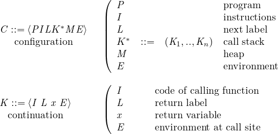


![[Decl ]
-I(L-) =-var-x =-e-M--E-e →-v----------
⟨PI LK ∗M E⟩−τ→ ⟨PI(L+1 )K∗M E [x ← v]⟩
[Drop ]
-I(L) =-drop-xτ---------------------
⟨PI LK ∗M E⟩− → ⟨PI(L+1 )K∗M E ∖{x}⟩
[ArrayDef ]
I(L ) = array x = [e1,..,en] M E e1 → v1 .. M E en → vn
a ∕∈ dom (M ) M ′ d=efM [a ← [v ,..,v ]]
---------------------τ-----1----n---------------------
⟨PILK ∗M E⟩ −→ ⟨PI(L +1)K ∗M ′E[x ← a]⟩
[ArrayDecl ]
I(L) = array x[e] M E e → n
a∈∕dom (M ) M ′ d=efM [a ← [nil1,..,niln]]
------∗------τ------------∗-′----------
⟨PILK M E⟩ −→ ⟨PI(L +1)K M E[x ← a]⟩
[Update ]
-I(L)-=-x-←-eτ--x-∈-dom(E)--M--E-e →-v
⟨PI LK ∗M E⟩− → ⟨PI(L+1 )K∗M E [x ← v]⟩
[ArrayUpdate ]
′ def ′
I(L) = x[e] ← e a = E (x) M E e → n M E e → v
M (ad)ef = [v0,..,vm] 0 ≤ n ≤ m
-M-′=-M-[a-←-[v0,..,vm]{vn∕v}]-----------------------
⟨PILK ∗M E ⟩−τ→ ⟨PI (L+1 )K ∗M ′E⟩
[Read ]
I(L) = readx
------------read lit----------------------
⟨PILK ∗M E ⟩ −→ ⟨PI(L +1)K ∗M E[x ← lit]⟩](main40x.png)
![[Print]
-I(L) =-printe--M--E-e →-lit--------
∗ print lit ∗
⟨PI LK M E⟩ − → ⟨PI(L+1 )K M E ⟩
[BranchT ]
-I(L) =-branch-e-L1L2--M--E-e →-true-
⟨PILK ∗M E ⟩−τ→ ⟨PI L1K ∗M E⟩
[BranchF ]
I(L) = branch e L1L2 M E e → false
---------∗------τ---------∗--------
⟨PILK M E ⟩−→ ⟨PI L2K M E⟩
[Goto ]
--I(L-) =-goto-L′-------------
⟨PI LK ∗ME ⟩−τ→ ⟨PIL′K ∗M E ⟩
[Stop ]
I(L) = stop
------------stop------------
⟨PI LK ∗M E⟩ −→ ⟨P𝜀LK ∗M E ⟩
[Call]
I(L ) = call x = e(e1,..,en)
M E e → F
P(F) = F(x1,..,xn) : DF I′ d=efP(F,active)
′ def ′ ′
-L-=-start(I)τ-M-E[x1 =-e1,..,xn =-en] ⇝-E----
⟨PI LK ∗M E⟩−→ ⟨PI′L′(K ∗,⟨I (L+1 ) x E⟩)M E′⟩
[Return ]
-I(L) =-returne-M--E-e-→-v----------------------
∗ ′ ′ ′ τ ′ ′ ∗ ′
⟨PI L(K ,⟨I L x E ⟩)M E⟩ −→ ⟨PI L K M E [x ← v]⟩](main41x.png)
![[AssumePass ]
-I(L) =-assume-e∗-else ξ-˜ξ∗-∀m,-M-E-em-→-true-
∗ τ ∗
⟨PI LK M E⟩− → ⟨PI(L+1 )K M E ⟩
[AssumeDeopt ]
∗ ˜∗
--I(L-) =-assume-eτ-else-ξξ---¬(∀m,-M-E-em-→--true)
⟨PI LK ∗M E⟩−→ deoptimize(⟨PILK ∗M E ⟩,ξ, ˜ξ∗)
[DeoptimizeConf ]
′ ′ def ′ ′
M EVA ⇝ E I = P(F ,V )
∀q∈ 1˜,..,r,
ξq = Fq.Vq.Lq xq VAqdef def
-----M-EVAq--⇝-Eq--Iq=--P(Fq,Vq)-Kq--=-⟨Iq-Lq-xq-Eq⟩---------------
deoptimize(⟨PILK ∗M E ⟩,F ′.V′.L′ VA, ˜ξ1,..,ξ ˜r) de=f⟨PI′L′(K ∗,K1,..,Kr)M E′⟩
[EvalEnv ]
M E e1 → v1 .. M E en → vn
M-E-[x-=-e-,..,x-=-e-] ⇝-[x--→-v-,..,x--→-v-]
1 1 n n 1 1 n n](main42x.png)
 (incl. previous 2
pages)
(incl. previous 2
pages) . The
. The 
![[StartConf ]
-I-d=efP-(main,active)-L-d=efstart(I)
start(P) de=f⟨PIL∅∅∅⟩
def T
reachable(P ) = {C | ∃T , start(P) −→ ∗ C }](main46x.png)


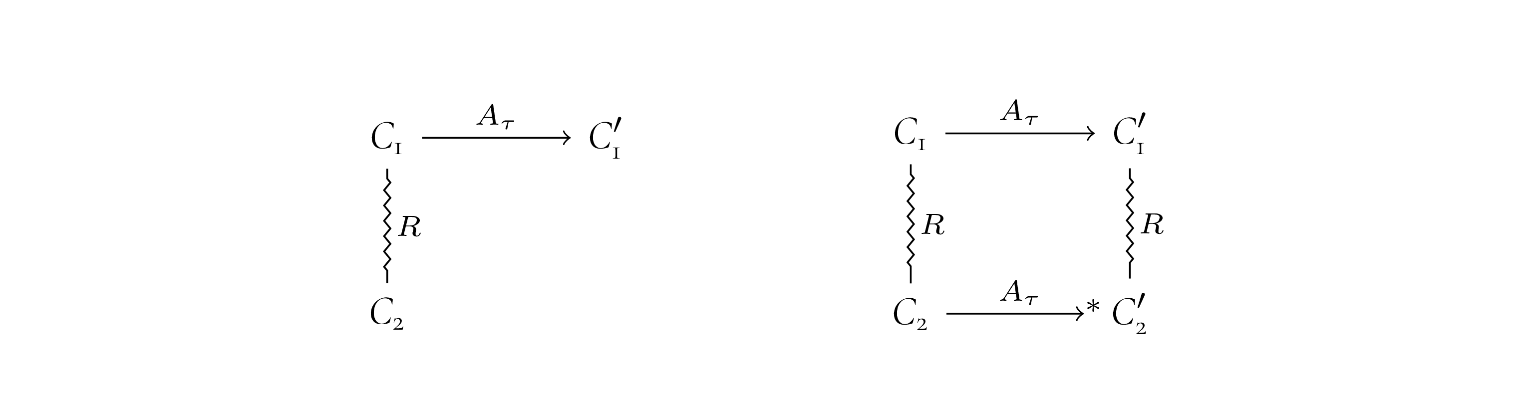
 (
(


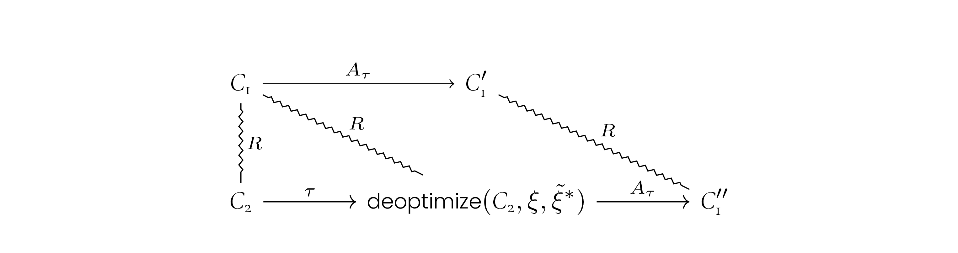 Let us first show that the reductions of


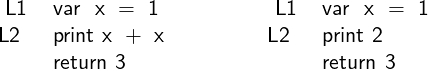
![def ∗
C1 = ⟨PP (F,V1 )L2K M [ x → 0 ]⟩
C2 de=f⟨PP (F,V2 )L2K ∗M [ x → 0 ]⟩](main87x.png)


 (
(


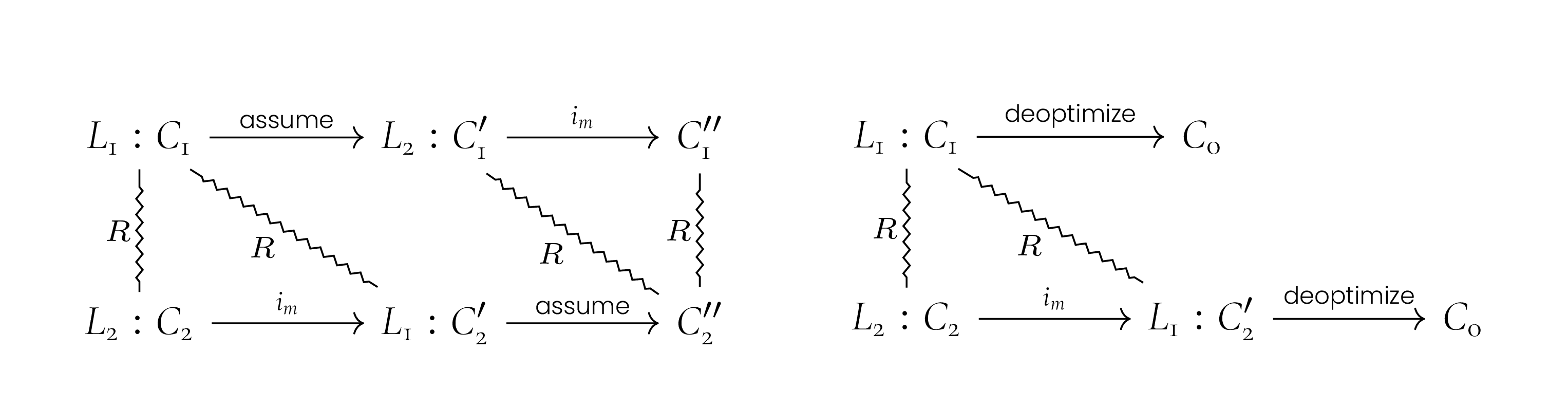


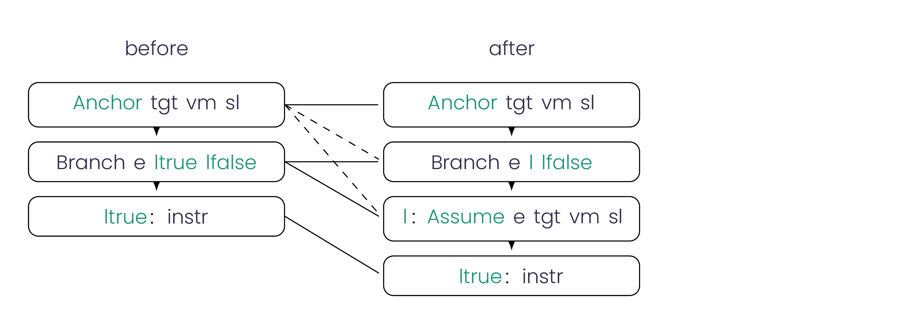

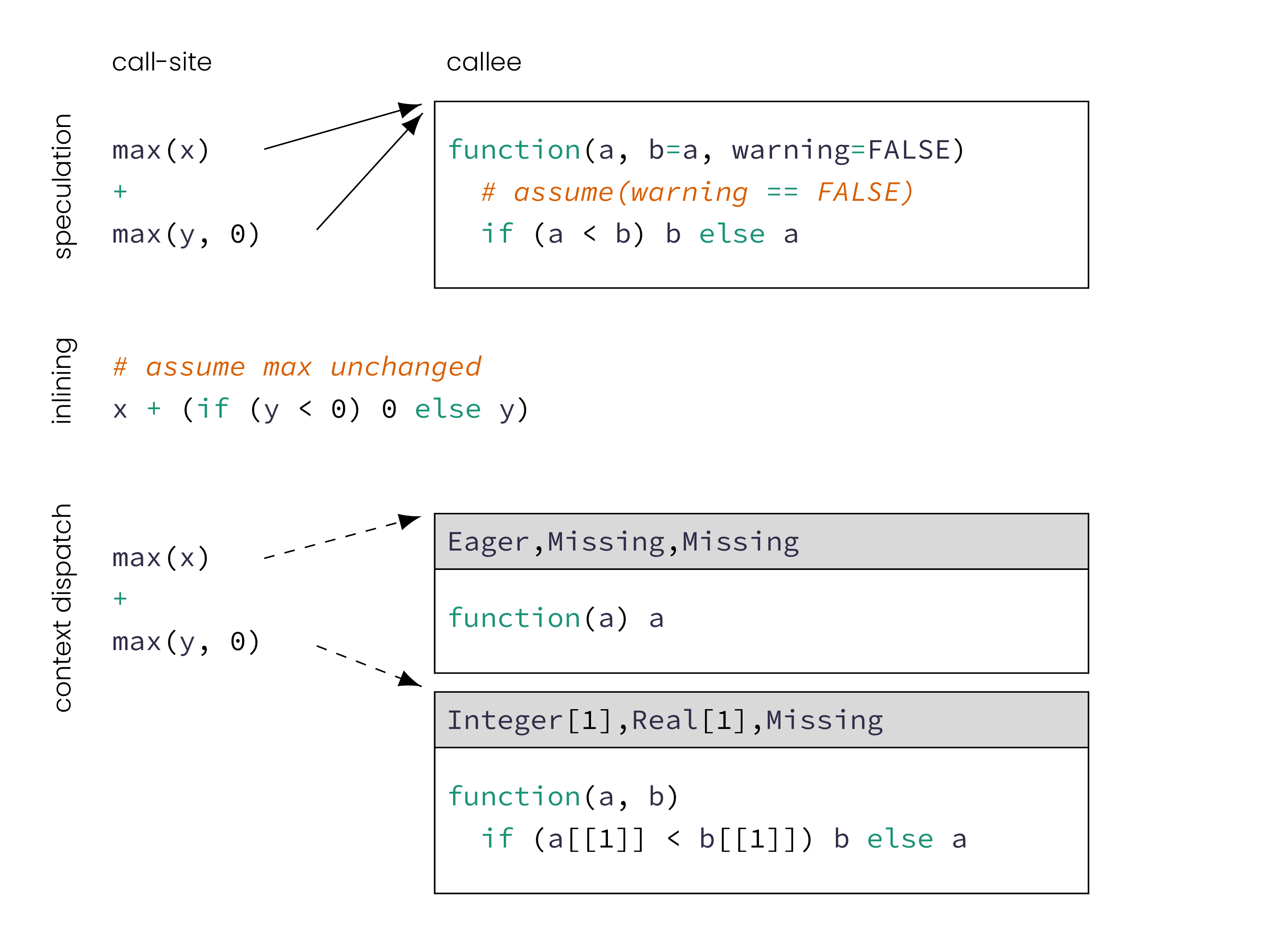
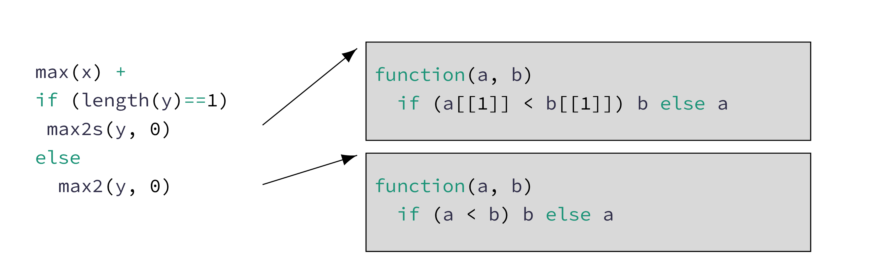
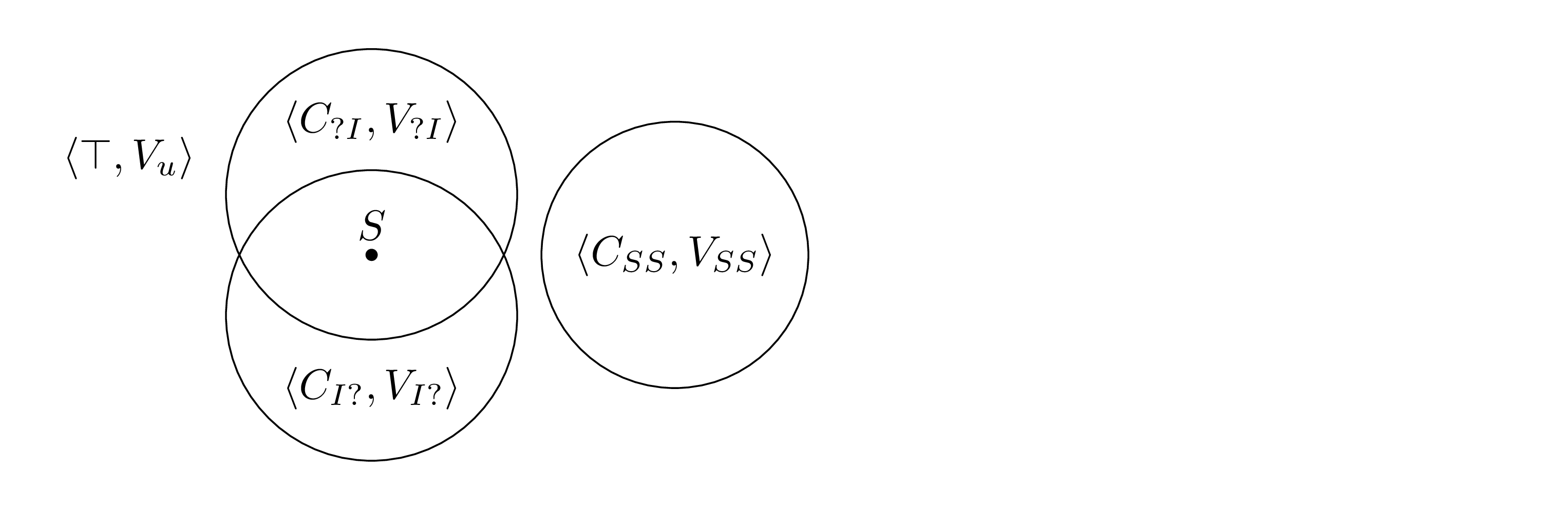
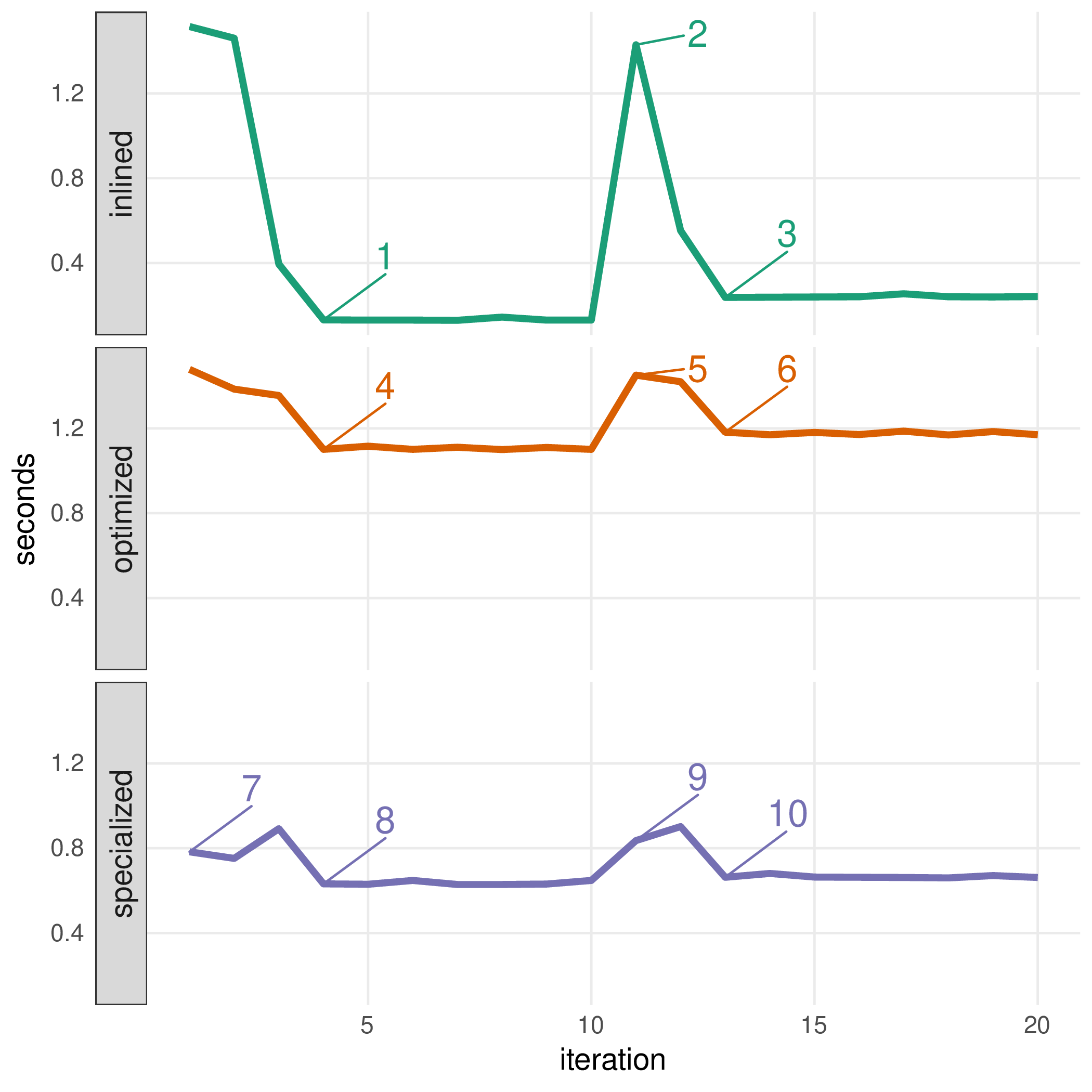
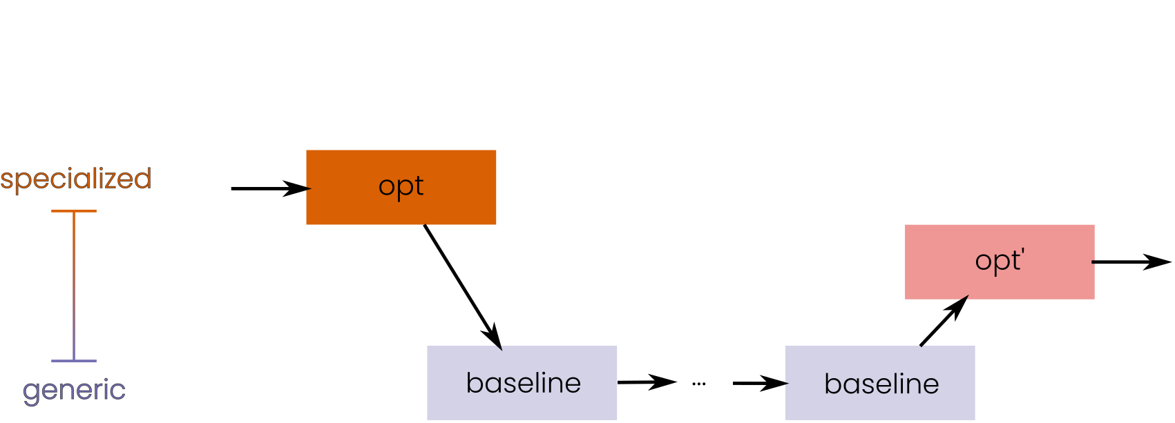
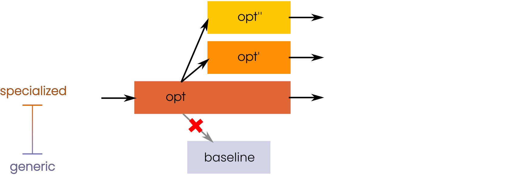
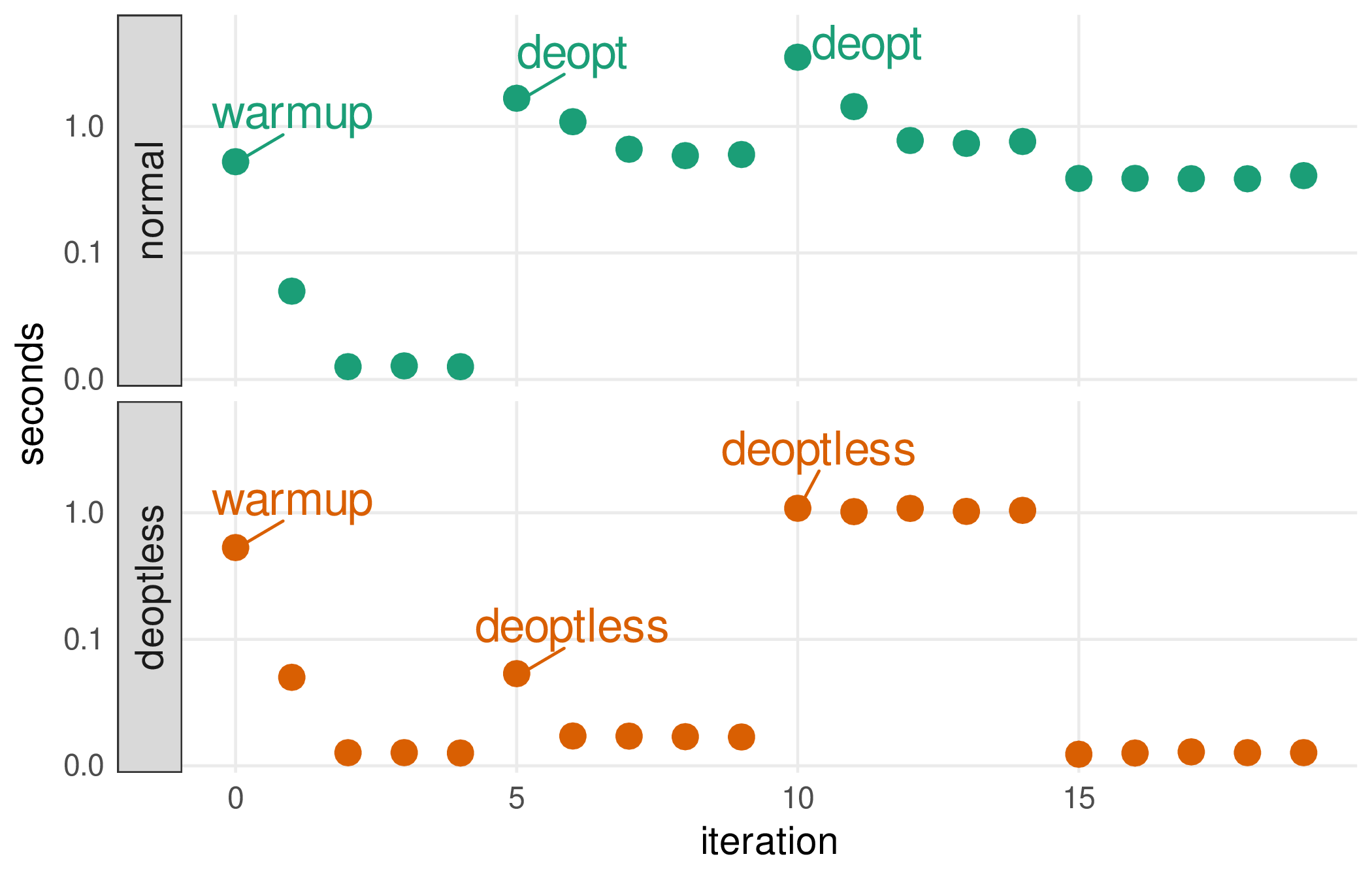
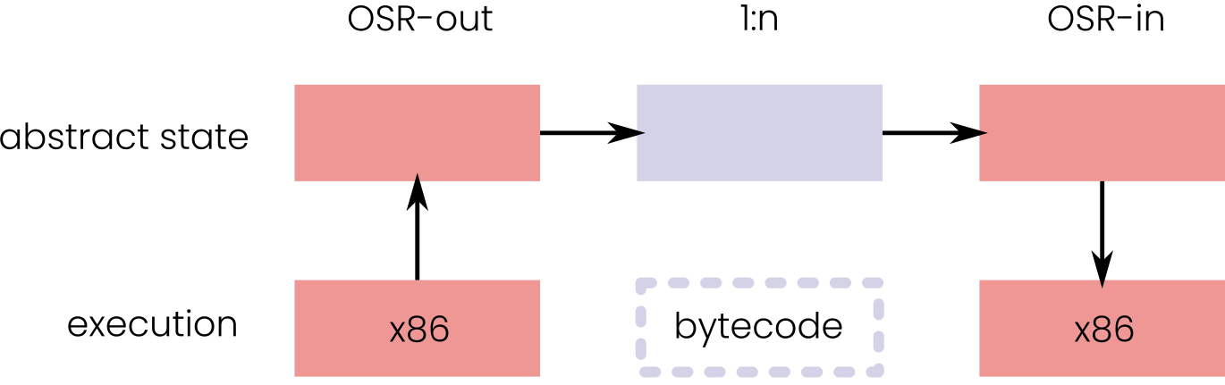
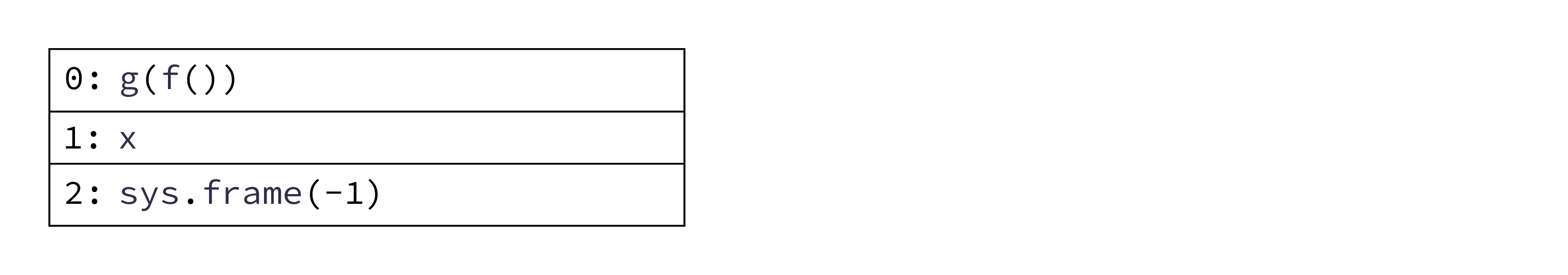
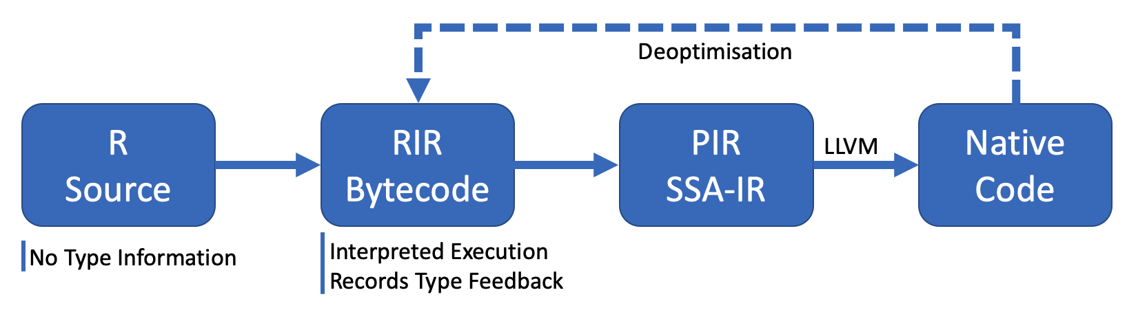
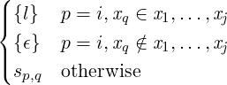
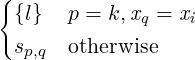
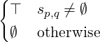
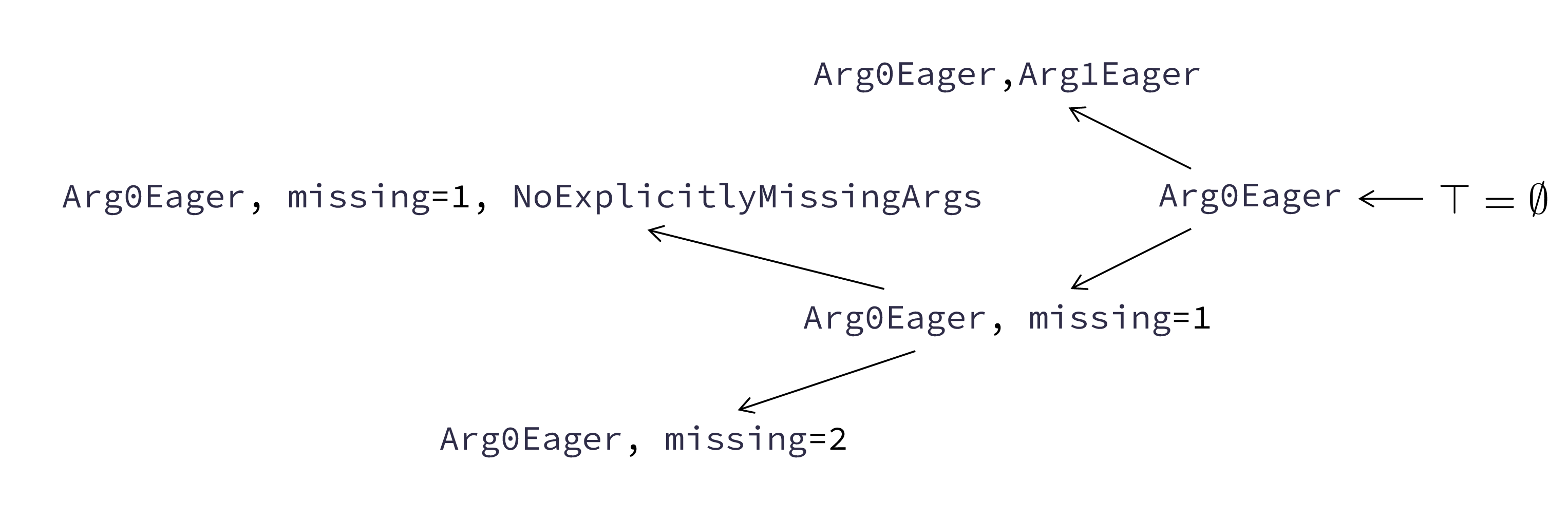
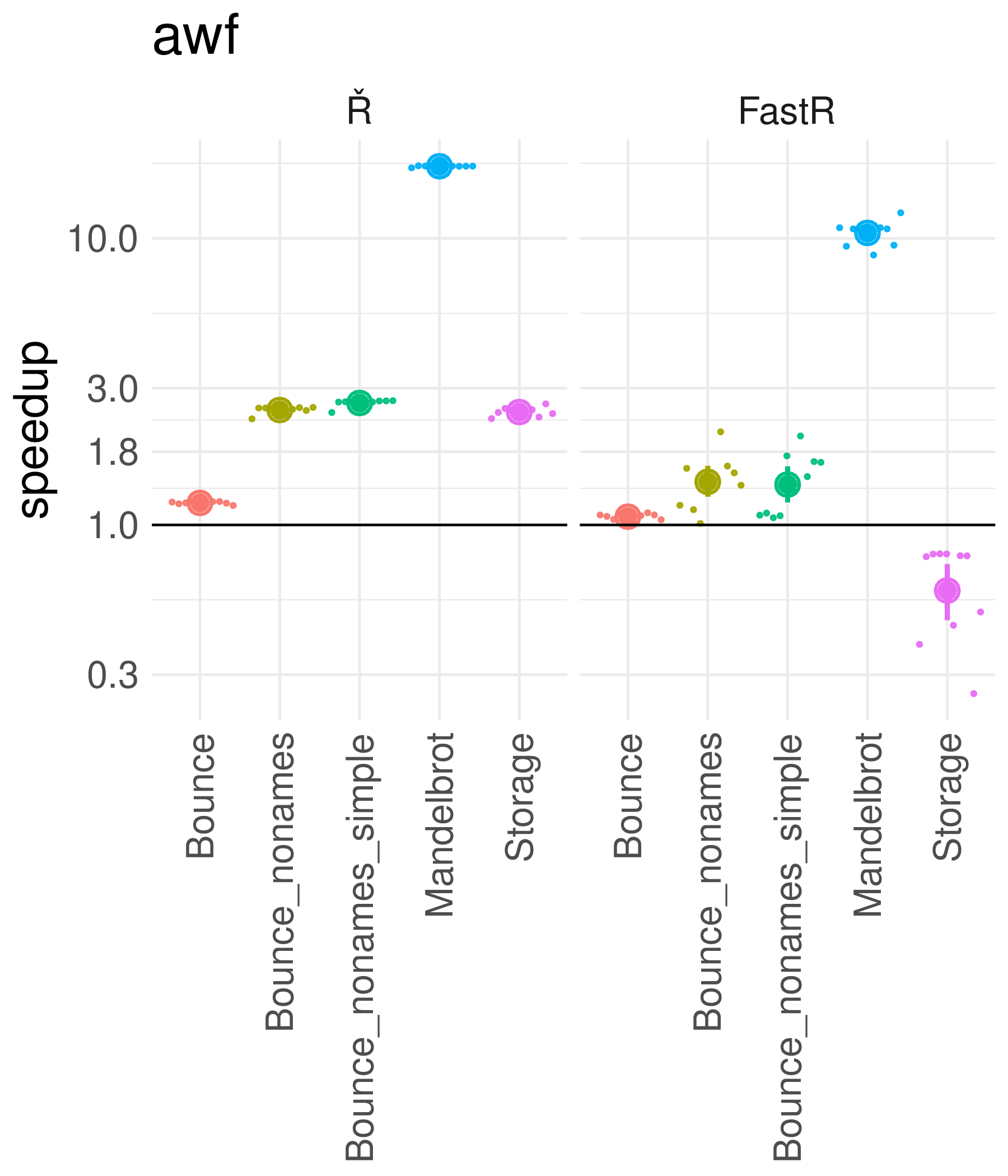
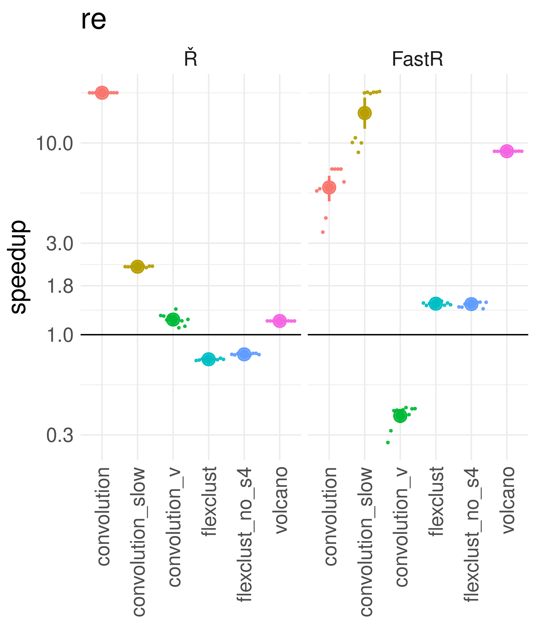
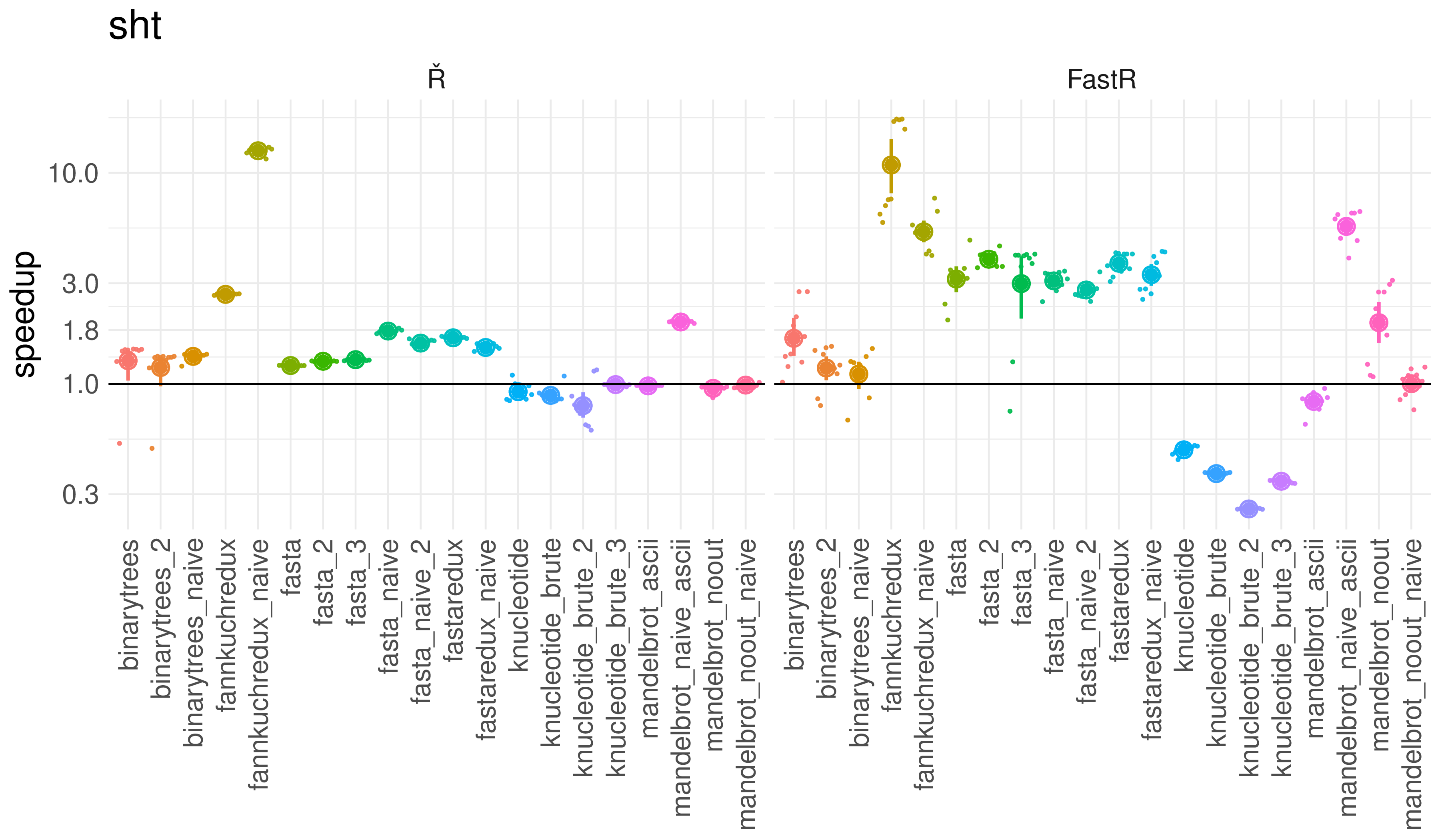
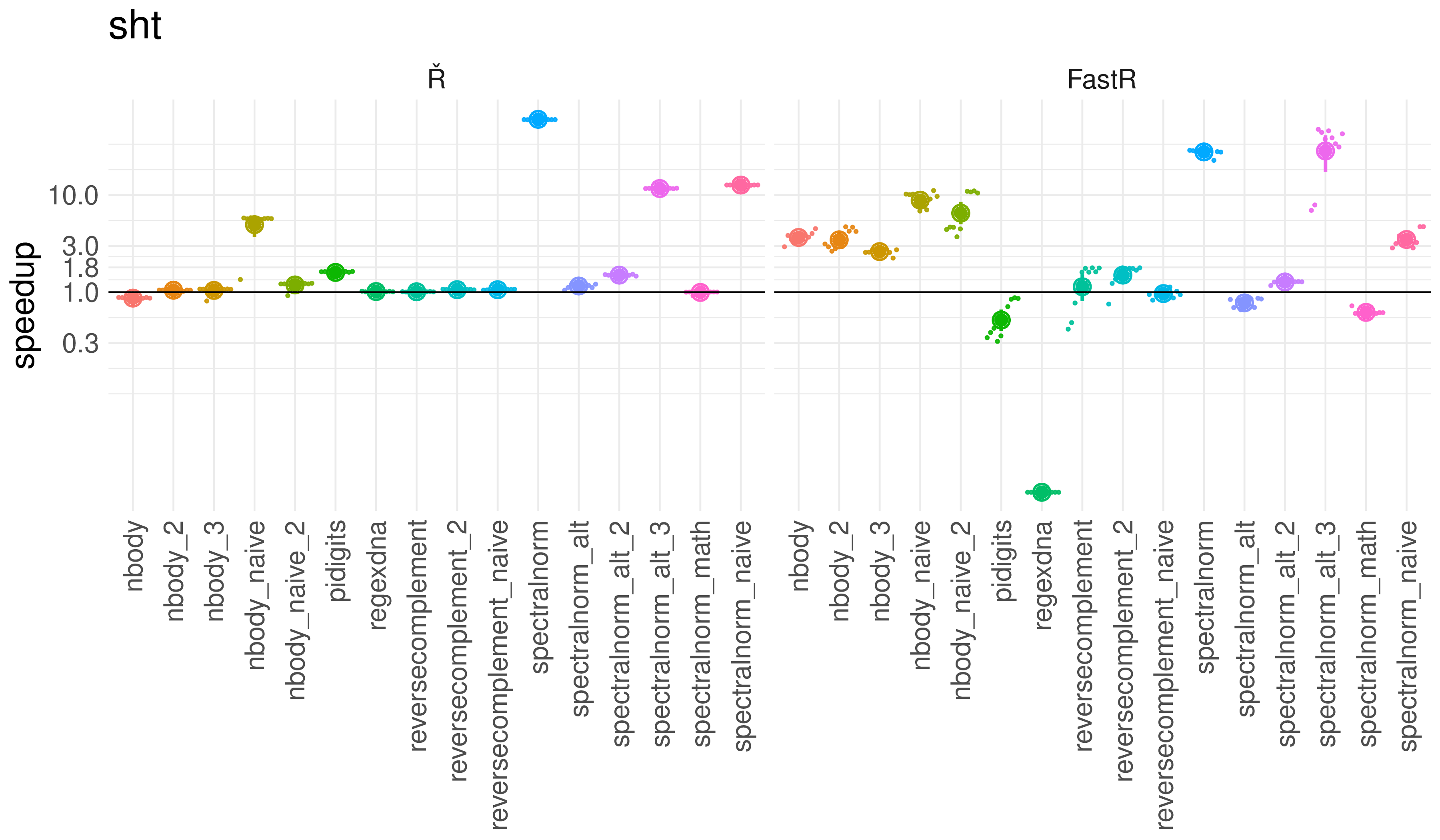
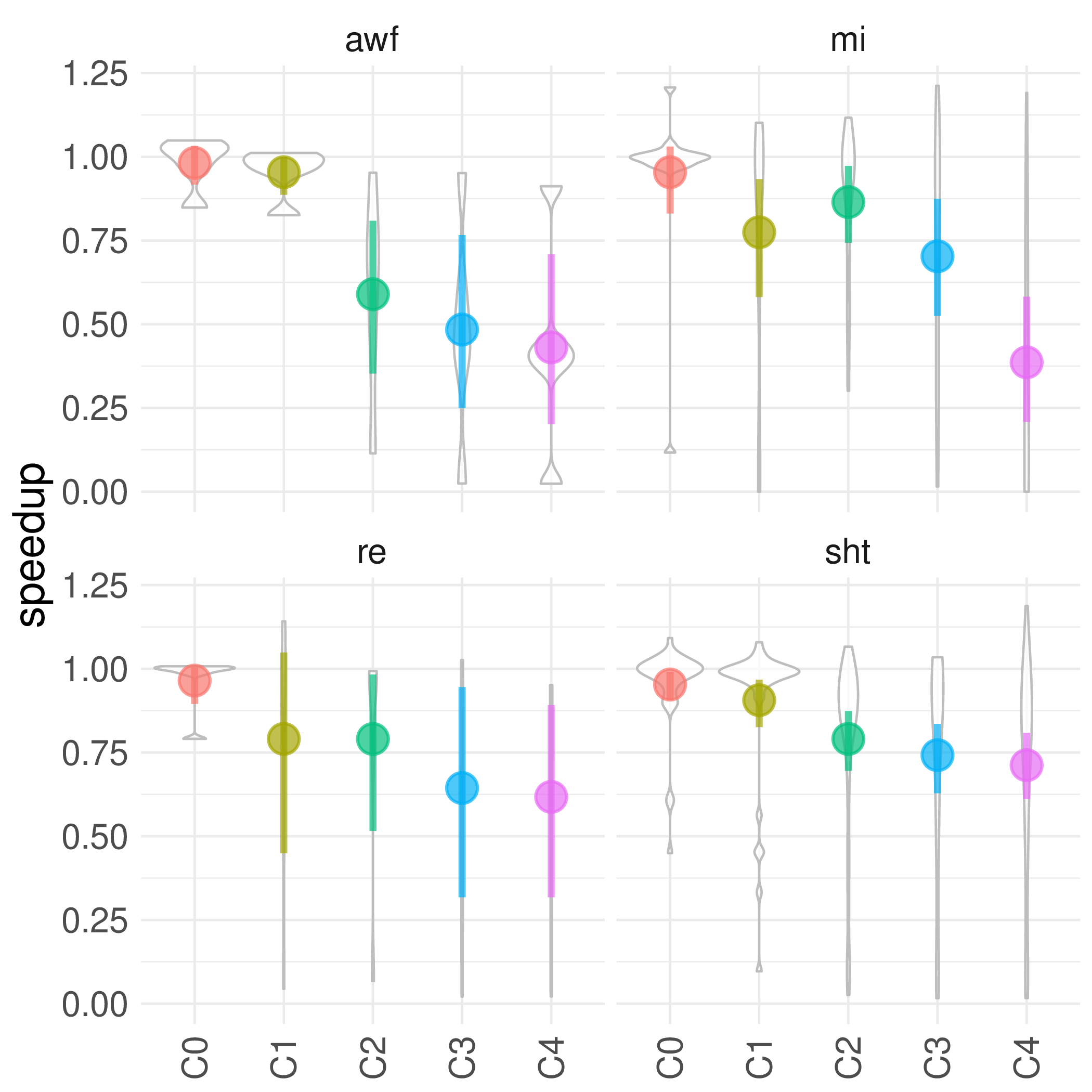
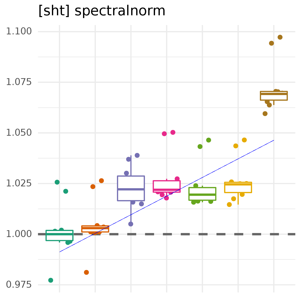
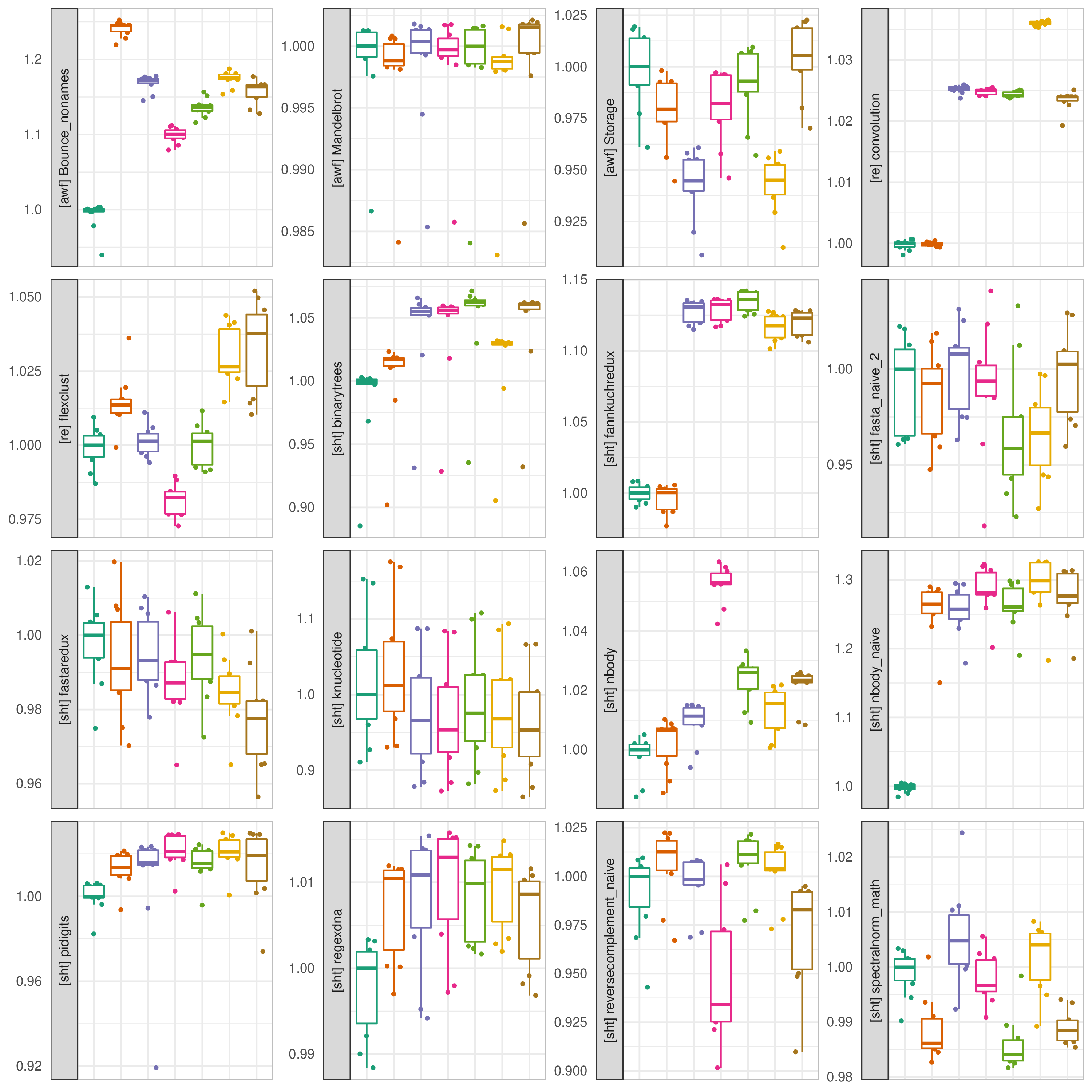
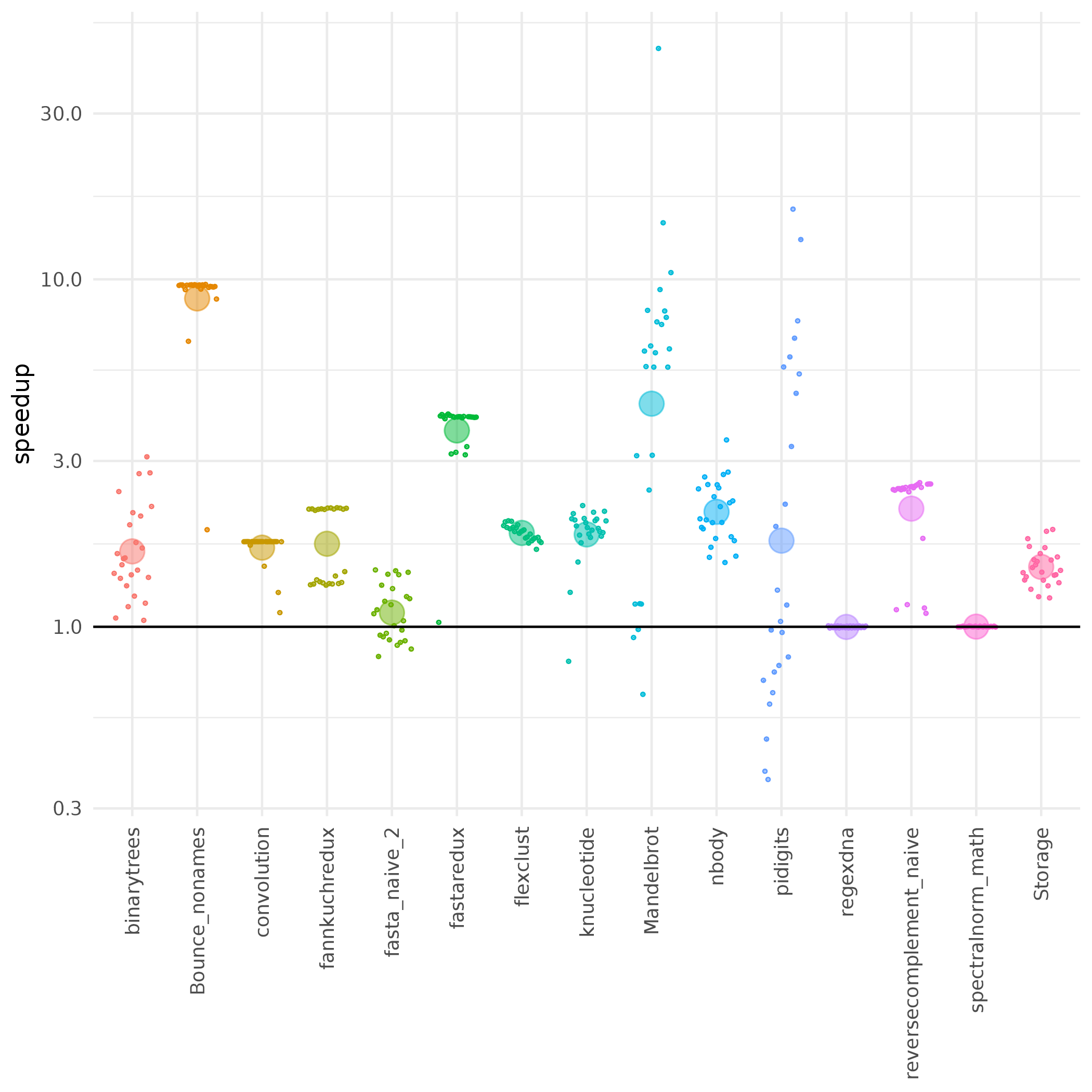
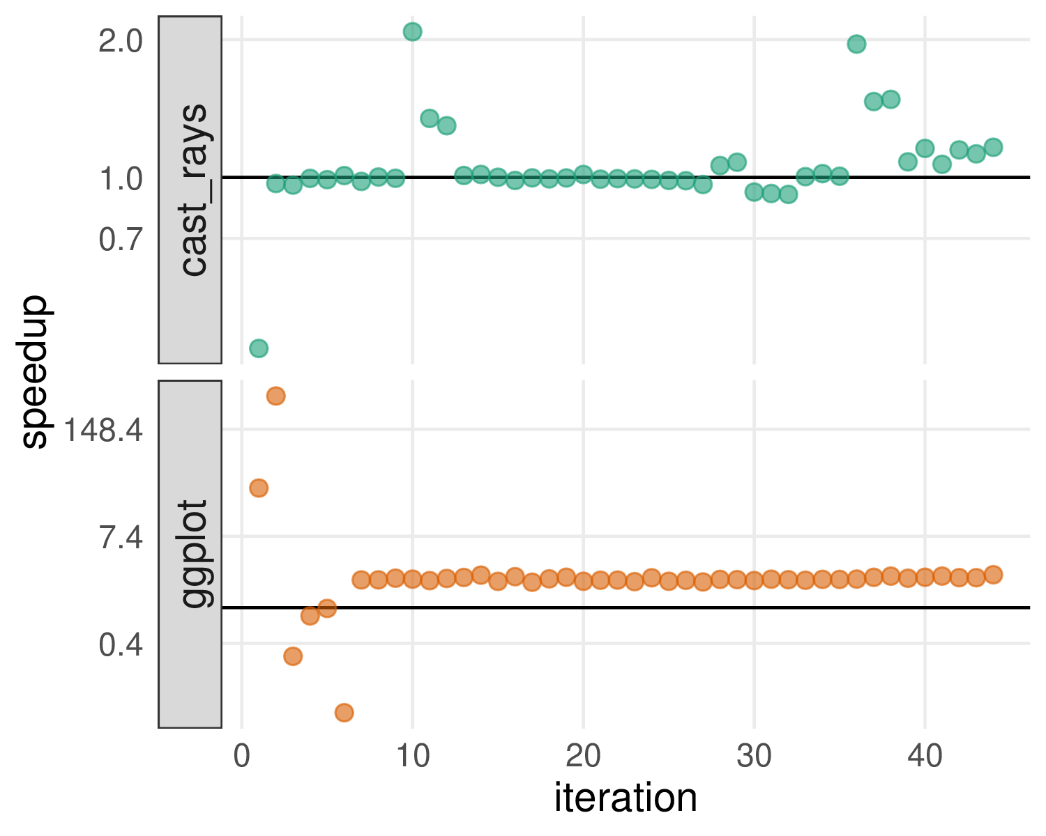
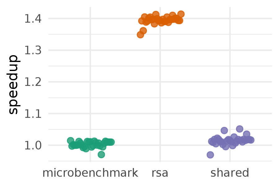
 of
expressions
of
expressions of simple expressions
 (incl.
previous 2 pages)
(incl.
previous 2 pages)![|
| assume x ⁄= nil else size.V b.L2 [ el = 32 , x = x ]
| var l = x [ 0 ]
| return l ∗ 32](main5x.png)
![|
L1 var el = 32
L2 branch x = nil L4 L3
L3 var l = x [ 0 ]
| return l ∗ el
L4 return 0](main6x.png)
![|
| assume x = 42 else show.V b.L1 [ x = x ]
| print 42](main7x.png)
![| assume true else show.V b.L1 [ x = 42 ]
|
| print x](main8x.png)

![|
L0 assume true else fun .V 1 .L0 []
| var x = 1
L1 assume e else fun.V 1 .L1 [ x = x ]
L2 print x + 2](main10x.png)
![|
L0 var x = 1
L1 assume e else fun.V 0 .L1 [ g = x ]
L2 assume true else fun .V 0 .L2 [ g = x , h = x + 1 ]
| print x + 2](main11x.png)
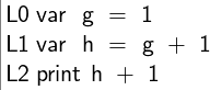
![|
L1 assume true else size.Vb.L1 [ x = x ]
| var el = 32
L2 assume true else size.Vb.L2 [ el = el , x = x ]
| branch x = nil L4 L3
L3 var l = x [ 0 ]
| return l ∗ el
|
L4 return 0](main13x.png)
![|
L1 assume true else size.Vb.L1 [ x = x ]
| var el = 32
L2 assume x ⁄= nil else size.V b.L2 [ el = el , x = x ]
| var l = x [ 0 ]
| return l ∗ el](main15x.png)
![|
array pl = [ 1 , 2 , 3 , 4 ]
array vec = [length( pl ), pl ]
var s = nil
var x = vec
assume x ⁄= nil else size.Vb.L2 [ el = 32 , x = x ]
| main.V b.Lret s [ pl = pl , vec = vec ]
var l = x [ 0 ]
|s ← l ∗ 32
|
drop l
drop x
print s
stop](main16x.png)
![|
| array pl = [ 1 , 2 , 3 , 4 ]
| array vec = [length( pl ), pl ]
| call s = size (vec)
Lretprint s
| stop
|](main17x.png)
![|
L2 assume x ⁄= nil else size.V b.L2 [ el = 32 , x = x ]
| var l = x [ 0 ]
| return l ∗ 32](main18x.png)
![| assume true else size.Vb.L1 [ x = x ]
| var el = 32
|
| branch x = nil L4 L3
L3 x ← x [ 0 ]
| return x ∗ el
L4 ...](main19x.png)
![| var x0 = x
| var el = 32
|
| branch x = nil L4 L3
L4 x ← x [ 0 ]
| assume x = 1 else size.Vb.L1 [ x = x0 ]
| return 1 ∗ el
L3 ...](main20x.png)
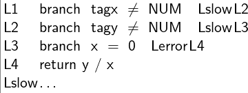

![v ::= values
| lit addr ::= a addresses
| F M ::= (a → [v1,..,vn])∗ heap
| a E ::= ( x → v)∗ environment](main23x.png)


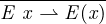
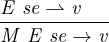
![E--se1-⇀-v1--..--E-sen-⇀-vn----------------
M E primop(se1,..,sen) → [[primop ]](v1,..,vn)](main28x.png)
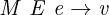 of expressions
![E--se-⇀-a--M-(a) =-[v1,..,vn]
M E length(se) → n](main30x.png)
![a d=efE (x) M (a) = [v0,..,vm ]
E--se-⇀-n--0-≤-n-≤-m--------
M E x[se] → vn](main31x.png)
 of simple expressions
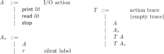

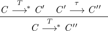
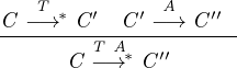
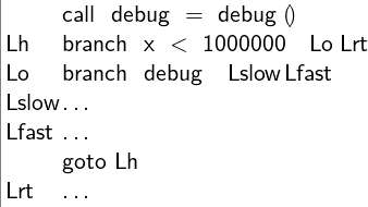
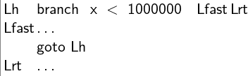
![|
L0 assume e1,e2,e3 else undo.Vs12.L0 [...]](main115x.png)
![|
L0 assume e1,e2 else undo .V s1.L0 [...]](main116x.png)
![|
L0 assume e1 else undo .V base.L0 [...]](main117x.png)